Doctrine Claim:
“It depends” is not a cop-out; it is the only honest answer to complex problems. But to be useful, you must follow it with what it depends on, the base rates of success, and the cost of being wrong. Most professional mistakes do not happen during routine work; they happen in the gap between “I’ve seen this before” and “I have no idea.” This doctrine provides the mental tooling to slow down, calculate odds, and act decisively when your pattern-matching fails. This guide turns vague uncertainty into structured precision.
Saying ‘it depends’ is not evasive if you explain what it depends on, why those factors matter, and what the probabilities actually are. This guide will show you how.
This page is a Doctrine Guide. It shows how to apply one principle from the Doctrine in real systems and real constraints. Use it as a reference when you are making decisions, designing workflows, or repairing things that broke under pressure.
“It depends” is not a cop-out; it is the only honest answer to complex problems. #
But to be useful, you must follow it with what it depends on, the base rates of success, and the cost of being wrong. Most professional mistakes do not happen during routine work; they happen in the gap between “I’ve seen this before” and “I have no idea.” This doctrine provides the mental tooling to slow down, calculate odds, and act decisively when your pattern-matching fails. This guide turns vague uncertainty into structured precision.
TL;DR: How To Use This Guide Without Drowning #
This guide is long on purpose. It is not meant to be consumed in a single sitting, unless you are very into this topic and have coffee. It is meant to be a one-stop reference so you do not have to jump between (twenty) five tabs, Wikipedia, and three old notes just to remember how to think about probability under uncertainty.
If you only have 3 minutes, start here.
The core idea #
Most mistakes do not happen in your everyday work.
Most mistakes happen when something is:
- High risk
- Low frequency
- And you actually have a little time to think
In those moments, the honest answer to “Will this work?” is usually:
It depends. Here is what it depends on, here is how likely each outcome is, and here is what it would cost to be wrong.
This guide shows you how to say that without sounding vague or weak.
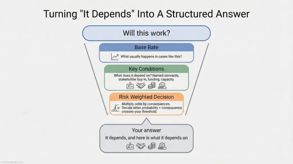
Working Rule – Say “It Depends” Like A Professional
Do not stop at “It depends.”
Follow it immediately with “Here is what it depends on, here is how the odds change under each condition, and here is what it would cost to be wrong.”
That turns a hedge into leadership.
What this guide does for you #
In one place, you get:
- A practical version of Bayesian reasoning
- Start with what usually happens (base rates)
- Update when new evidence shows up
- Ask what the outcome depends on (conditions)
- Weight probability by consequences, not just odds
- A vocabulary crosswalk
- What you already say in real life
- The formal term someone might use
- Concrete examples from fire, systems integration, and career decisions
- Ready to use snippets and rules
- Simple tests like “What usually happens?” and “Which error costs more?”
- Phrasing you can drop into emails, briefs, or interviews
You do not need the math. You get the patterns, language, and examples.
How to read this if you are new here #
If you are not me and you just landed on this page, try this route:
- Read Section 1
Get the High Risk / Low Frequency matrix into your head. That tells you where mistakes cluster. - Skim Sections 2 to 5
Look for the bold headings and the small tables that say “What you say / Formal term / Example.” That gives you the vocabulary. - Read Section 15 and Section 16
These two sections tell you when to trust your patterns and when to slow down, and give you a checklist you can actually use. - Pick one field example in Section 17
Choose the story that is closest to your world and read only that one. Do not feel obligated to read every example.
You can come back later for the rest. This is a shelf reference, not a social media post.
How to use this if you are me #
If you are future me, here is why this page exists:
- It gives me a single canonical place to pull:
- Slides on risk frequency
- Soundbites for “it depends” that do not sound weak
- Examples for interviews, training, and doctrine videos
- It goes one level deeper than you usually see online
- When you mention Bayes, expected value, or survivor bias on camera, you can grab definitions and micro stories from here without leaving the site.
Opening: Most of What You Do Goes Right #
Most of what you do goes right.
Think about that for a second. In spite of the extremely complex nature of your job (hundreds or thousands of things to manage, high stakes, incomplete information, time pressure), most of what you do, you do right.
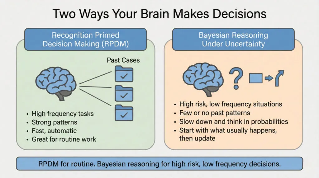
Why? Because your brain is a massive pattern-matching engine. Gordon Graham, a legendary fire service trainer, calls it “Recognition Primed Decision Making” or RPDM. When you encounter a situation, your brain scans past experience, finds a match, and automatically directs behavior based on what worked before.
RPDM works great for high-frequency events. Things you do all the time. Your “hard drive” or pattern library is full of past cases. Pattern matching is reliable and extensive.
But RPDM fails on high-risk, low-frequency events. Things you do rarely but where consequences are severe. Your hard drive is empty. No past pattern to match. You can learn more about RPDM and low-frequency/high impact events in this YouTube Video (local copy below to prevent link rot)
That’s when mistakes happen.
Graham’s advice for these situations: Slow down. If you have time on a task, use it. Don’t rush high-risk, low-frequency decisions as if they were routine.
This guide teaches you how to slow down and think it through. The formal term is “Bayesian reasoning” (a way of making decisions under uncertainty by starting with what usually happens, updating based on specific evidence, and weighting probabilities by consequences).
You already do this intuitively. This guide just gives you vocabulary and structure for reasoning you already use, so you can explain your thinking to people who demand “yes or no” when the right answer is “it depends, and here’s why.”
Note: If you want to read more on the model and research behind RPDM, look up the works of Gary Klein (wikipedia). The Recognition Primed Decision (RPD) model was introduced by klein and his colleagues to explain how experts make rapid, effective decisions under pressure in real-world, naturalistic settings, which was something traditional decision-making models didn’t adequately cover.
A Brief Note on History #
The mathematical foundation for this thinking comes from Reverend Thomas Bayes, who developed what’s now called “Bayes’ theorem” in 1763. The theorem shows how to update probability estimates when new evidence arrives. Since then, Bayesian reasoning has become fundamental to statistics, machine learning, decision theory, and scientific inference.
But experienced operators have been using this reasoning pattern for centuries (long before anyone formalized the math). An incident commander updating fire containment odds based on changing wind conditions is doing Bayesian reasoning, whether they know the formal term or not. A program manager adjusting integration success estimates after learning a partner has named stewards is doing Bayesian reasoning. A systems architect saying “it depends on stakeholder buy-in” is thinking conditionally, which is the foundation of Bayesian probability.
This guide gives you vocabulary for reasoning you already use. You don’t need to know the math. You just need to recognize the patterns in your own thinking so you can explain them to people who want certainty when the honest answer is uncertainty with structure.
Section 1: The Risk-Frequency Matrix (Where Mistakes Happen) #
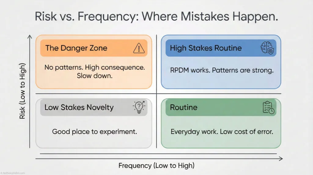
Gordon Graham teaches firefighters to think about every task they do through a simple framework: Risk and Frequency.
Some things you do are high risk (if they go wrong, consequences are severe). Some things are low risk (consequences are small even if they fail). Some things you do all the time (high frequency). Some things you do rarely (low frequency).
Put these together and you get four boxes:
Risk Frequency Matrix: Where Mistakes Actually Happen #
Every task you touch sits somewhere on a grid of Risk and Frequency. Most of what you do is either low risk or high frequency, so your patterns carry you. The trouble starts in one quadrant in particular.
High Risk / Low Frequency (Danger Zone) #
This is where most serious mistakes live.Your "hard drive" is empty, you have no patterns to lean on.Stakes are severe and you cannot afford a casual guess.If you have discretionary time, this is where you slow down and think in probabilities.
Low Risk / Low Frequency #
Rare tasks with small consequences.You can experiment and learn without big downside.Good place to prototype new patterns and training.
High Risk / High Frequency #
You run these often and the stakes are high.Patterns are strong and procedures exist.RPDM usually works here. It may be "routine," but you still respect the risk because it is a known known.
–
Low Risk / High Frequency #
Routine work, done all the time, with small consequences.RPDM carries the load and error cost is low.You do not need Bayesian framing for most of this.
Most of your visible effort lives in the safe quadrants. Most of your catastrophic surprises come from the top right: high risk, low frequency, with a little bit of time to decide. This guide is written for that box.
Where do mistakes happen?
Very rarely on high-frequency events (high or low risk). Why? Because you do them all the time. RPDM handles it. Your brain has seen this pattern hundreds of times and knows what works.
Not much on low-risk events (high or low frequency). Why? Because even if they go bad, the consequences are small. You can afford to be wrong.
Where mistakes happen: High risk, low frequency. The danger zone.
Graham calls these “the ones that scare the hell out of me.” High consequence, low probability. You don’t do them often enough to have strong patterns. But when they go wrong, the consequences are severe.
Working Rule – Slow Down In The Danger Zone
If something is both high risk and low frequency and you have any discretionary time at all, slow down.
This is not a pattern match problem. It is a probability and consequence problem.
Examples from Graham’s world:
- JFK Jr. flying at night in fog with 170 hours of flight time (high risk, low frequency)
- Boulder PD handling the JonBenet Ramsey case (child homicide, high risk, low frequency)
- Seattle PD handling WTO riots (high risk for them because low frequency, but high frequency for LAPD who handles riots regularly)
Examples from your world (wherever you work):
- Panel interview for job you really need (high stakes, don’t do often)
- First time deploying to major disaster (high consequence, no past experience)
- System integration across agencies you’ve never worked with (high risk, novel situation)
- Presenting to executive board on topic outside your usual domain (high stakes, unfamiliar format)
Your hard drive is empty. No strong pattern to match. RPDM doesn’t help you here.
That’s when you need to slow down and think it through. That’s when Bayesian reasoning matters.
Section 2: Base Rates (What Usually Happens) #
You already talk in base rates. You just do not call them that. Here is the translation so you can move cleanly between operator language and formal vocabulary.
The first question in any Bayesian analysis: What usually happens in situations like this?
The formal term is “base rate.” It’s the overall probability of something happening before you know any specific details about this particular case. It’s your starting point.
When a program manager asks “How often do integrations like this succeed?”, they’re asking for the base rate. The answer might be “70% fail” or “30% succeed.” That’s your starting estimate before you know anything specific about THIS particular integration.
The Crosswalk: #
| What You Say | Formal Term | Example |
|---|---|---|
| “What usually happens in situations like this?” | Base rate | “70% of integrations between federal agencies fail” |
| “Based on past experience…” “Based on past experience, this usually goes sideways.” | Prior probability | “We tried this 10 times, succeeded 3 times” |
| “In situations like this…” “In this kind of forced integration, it rarely works without buy in.” | Reference class | “Integrations where leadership pushes it but stakeholders are not actually committed.” |
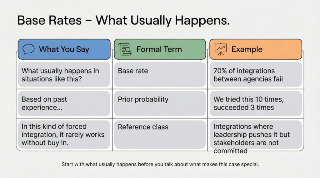
Working Rule – Start With What Usually Happens
Before you talk about what makes “this” case special, say what usually happens in situations like this.
That is your base rate. Everything else is an adjustment.
Why Base Rates Matter: #
Common mistake: Base rate neglect. People ignore overall patterns and focus only on specific details.
Rule: Before you talk about what makes this case special, say out loud what usually happens in cases like this. That is your base rate.
Example:
- Base rate: 90% of startups fail
- Specific detail: “But this founder is really passionate!”
- Wrong thinking: Passion overrides 90% failure rate
- Right thinking: Start with 90% failure, then ask “Does passion significantly change these odds?” (usually not much)
Field example from systems integration:
Wrong: “This integration will work because we have executive buy-in.”
- Ignores base rate (70% of integrations fail even WITH executive buy-in)
Right: “Integrations fail 70% of the time. Executive buy-in improves odds to maybe 40% success. We also have named stewards, which pushes it to 60% success. Still risky, but better than base rate.”
- Starts with base rate, then adjusts based on specific evidence
The Rule: #
Always ask “What usually happens in situations like this?” BEFORE you consider what makes this situation special. Don’t let specific details blind you to overall patterns.
When someone says “this time will be different,” your first question should be: “Different from what base rate? And what evidence makes you think the odds changed?”
You can call this “checking the base rate” or just “looking at what usually happens.” Either way, don’t skip this step.
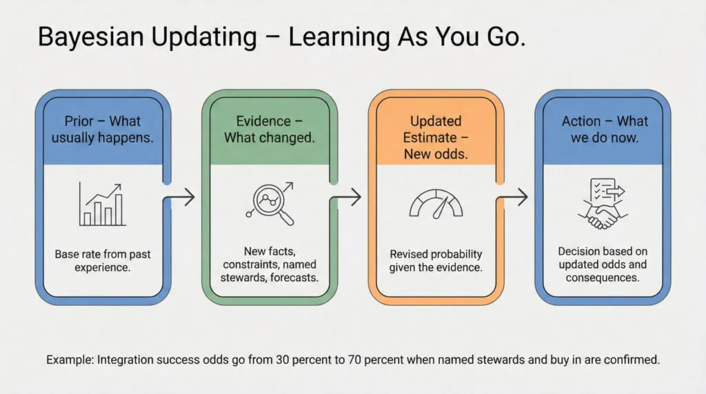
Section 3: Bayesian Updating (When New Evidence Changes Your Estimate) #
The formal term is “Bayes’ theorem” or “Bayesian updating,” named after Reverend Thomas Bayes who developed the mathematical foundation in 1763. The theorem shows how to revise probability estimates when new evidence arrives.
But you don’t need the math to use the thinking pattern.
What It Looks Like in Practice: #
When an incident commander says “The forecast changed, so our containment odds just dropped,” they’re doing Bayesian updating. They started with one probability estimate, new evidence (weather forecast) arrived, and they revised their estimate.
When a hiring manager says “I was skeptical about this candidate, but after seeing their portfolio, I’m more confident,” they’re doing Bayesian updating.
When you say “We tried integration before and it failed 7 out of 10 times, but this partner has a named steward, so I’m more optimistic this time,” you’re doing Bayesian updating.
The Pattern: #
- Start with prior probability (what usually happens, or past experience)
- New evidence arrives (forecast changes, partner capabilities become clear, constraints emerge)
- Calculate posterior probability (updated estimate given new evidence)
- Act on updated estimate
The Crosswalk: #
| Formal Term | Practitioner Language | Example |
|---|---|---|
| Prior probability | “What usually happens” or “Based on past experience” | “Integration usually fails 70% of the time” |
| Likelihood | “How much this evidence changes things” | “But with named stewards, success rate is 70%” |
| Posterior probability | “Updated estimate given new info” | “So for THIS integration, I estimate 70% success” |
| Bayesian updating | “Learning as you go” or “Revising estimate based on evidence” | “Was 30%, now 70% given new information” |
Why This Matters: #
You’re not being wishy-washy when you change your estimate based on new evidence. You’re being accurate. Ignoring new evidence is stubborn, not confident.
The person who says “I estimated 30% success last week and I’m sticking with that” even after learning critical new information (named steward, stakeholder buy-in, funding secured) is not being principled. They’re being stuck.
The person who says “I estimated 30% success last week, but we now have a named steward and stakeholder buy-in, so I’m revising to 70% success” is updating their beliefs based on evidence. That’s rational.
You can call this “Bayesian updating” in formal settings, or just “learning as you go” in field settings. Either way, you’re doing it right.
Section 4: Conditional Probability (It Depends on Context) #
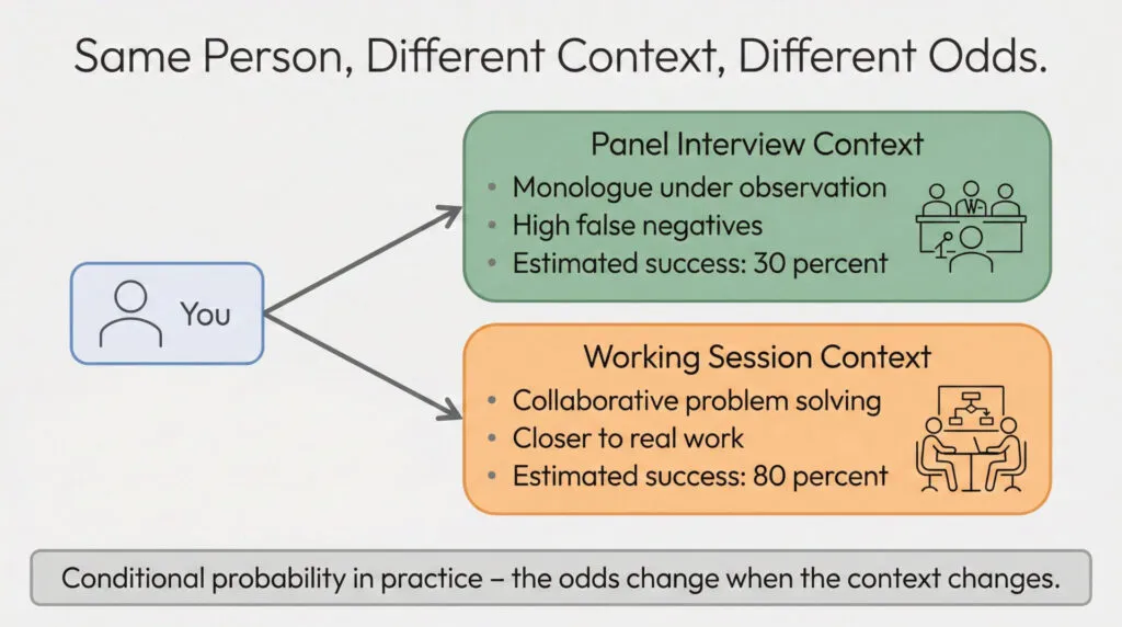
Here’s the thing about panel interviews. They test for one specific skill: unstructured monologue performance under observation.
But the actual work requires something different. Stakeholder dialogue. Collaborative problem-solving. Building systems iteratively with partners.
Same person. Different context. Different odds.
This is conditional probability. The formal term is P(A|B), which reads as “probability of A given B.” It means the probability of an outcome changes depending on the conditions.
What It Looks Like in Practice: #
When you say “It depends on wind speed and fuel moisture,” you’re thinking conditionally. The probability of containing the fire changes based on specific conditions.
When you say “Will this integration work? Depends on whether we have named stewards,” you’re thinking conditionally.
When you say “I’m great at collaborative work but struggle in panel interviews,” you’re recognizing that your success probability changes based on evaluation format.
The Crosswalk: #
| What You Say | Formal Term | Example |
|---|---|---|
| “It depends on…” | Conditional probability P(A|B) | “Depends on stakeholder buy-in” |
| “In this context…” | Conditioning on specific conditions | “In panel interviews vs actual work” |
| “Same action, different setting, different result” | Context-dependent probability | “I excel in dialogue, struggle in monologue” |
Examples: #
System Integration Success:
- P(success | no steward, no buy-in) = 10%
- P(success | named steward, no buy-in) = 40%
- P(success | named steward, stakeholder buy-in) = 70%
Same integration goal. Different conditions. Different odds.
Interview Performance:
- P(success | panel interview, behavioral questions, no cues) = 30%
- P(success | working session, collaborative problem-solving, dialogue) = 80%
Same person. Different evaluation format. Different odds.
Disaster Deployment:
- P(success | heroics-dependent system, no capacity plan) = 40%
- P(success | capacity-based system, named stewards, documented procedures) = 80%
Same mission. Different system design. Different odds.
Why This Matters: #
When someone asks “Will this work?”, the honest answer is almost never “yes” or “no.” The honest answer is “It depends, and here’s what it depends on.”
That’s not uncertainty. That’s accuracy. You’re recognizing that outcomes change based on conditions.
The person who says “yes, it will work” without specifying conditions is either overconfident or hasn’t thought it through. The person who says “it depends on named stewards, stakeholder buy-in, and funding” is giving you actionable information.
You can call this “conditional probability” or you can just call it “it depends.” Either way, you’re right to think this way.
Section 5: Expected Value: Why You Evacuate At Thirty Percent (Risk-Weighted Decisions) #
Not all outcomes have equal consequences.
–>Expected value means you care about Probability multiplied by Consequence, not just the odds by themselves.
- A low probability with catastrophic downside can be more important than a high probability with trivial cost.
- This is why it is rational to evacuate at thirty percent hurricane odds. You are trading a likely small cost now for protection against a rare but huge loss.
- When you say “Even if it is unlikely, we cannot afford to be wrong,” you are doing expected value in plain language.
Rule: Multiply how likely something is by how bad it would be if you were wrong. If that number feels bigger than your comfort threshold, act, even if the raw probability looks low.
This is why you evacuate at 30% hurricane probability. The 70% chance it misses doesn’t matter as much as the catastrophic cost if it hits.
The formal term is “expected value.” It means you weight probability by consequences, not just look at probability alone.
The Framework: #
Expected Value = Probability × Consequence
Or more precisely: Sum of (Probability of each outcome × Value of that outcome)
Example: Evacuation Decision #
- P(hurricane hits) = 30%
- Cost of evacuating unnecessarily = $10,000 (hotel, lost work time, hassle)
- Cost of NOT evacuating when hurricane hits = $500,000 (property loss, injury, death)
Expected value of evacuating:
- (70% × $10,000 cost) + (30% × $0 loss from hurricane) = $7,000 cost
Expected value of NOT evacuating:
- (70% × $0) + (30% × $500,000 loss) = $150,000 expected loss
Even though hurricane is unlikely (30%), expected value says evacuate. The asymmetry in consequences overwhelms the probability.
The Crosswalk: #
| What You Say | Formal Term | Example |
|---|---|---|
| “Even if it’s unlikely, the consequences are too severe to risk” | Expected value / Risk weighting | Evacuate at 30% hurricane odds |
| “Probably won’t happen, but if it does we’re screwed” | Tail risk | Low probability, catastrophic consequence |
| “Not worth the risk even if odds are in our favor” | Asymmetric payoff | 70% success but failure = mission critical loss |
| “We can’t afford to be wrong on this” | High cost of false negative | Miss a real problem = disaster |
Why This Matters: #
Gordon Graham teaches firefighters to “study the consequences.” Don’t just think about probability. Think about what happens if you’re wrong.
High-risk, low-frequency events are dangerous not just because your hard drive is empty (probability estimation is hard), but because the consequences of being wrong are severe.
Example from systems work:
Wrong thinking: “There’s only a 10% chance this integration will fail catastrophically, so we should proceed.”
Right thinking: “There’s a 10% chance this integration fails catastrophically. If it fails, we lose $5 million and mission-critical capability for 6 months. Expected cost of failure = 10% × $5M = $500K. Is the benefit of success worth a $500K expected loss? Do we have ways to reduce the 10% failure probability or mitigate the $5M cost?”
Weight probability by consequences, not just probability alone.
When To Act on Low-Probability Events: #
Act when: Probability × Consequence > Threshold
Even 10% probability matters if consequence is catastrophic. Even 90% probability might not justify action if consequence is trivial.
This is why you take low-probability, high-consequence threats seriously (pandemic preparedness, infrastructure failure, security breaches). Not because they’re likely. Because you can’t afford to be wrong.
Section 6: False Positives and False Negatives (Evaluation Errors) #
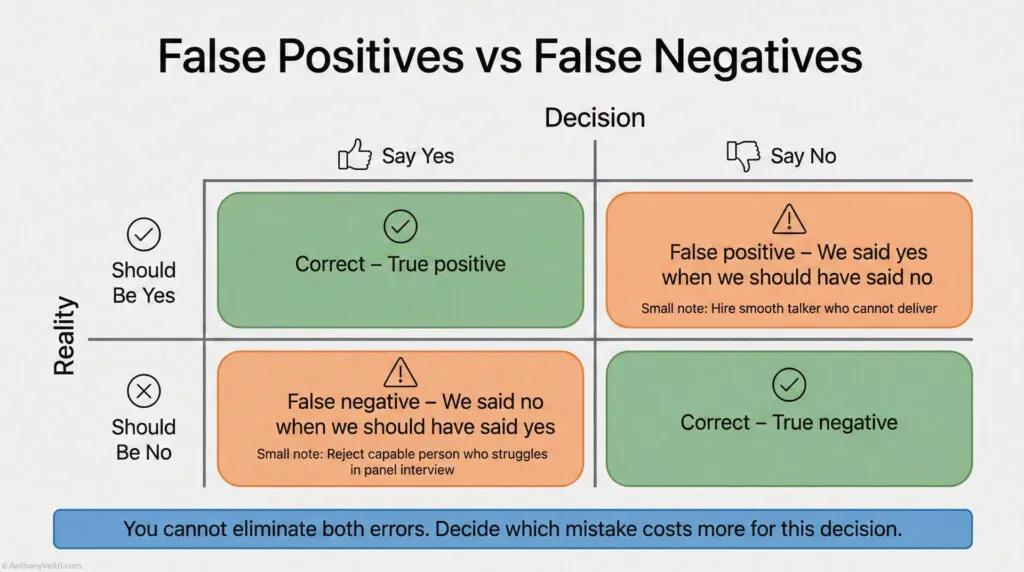
There are two ways an evaluation can be wrong:
False positive (Type I error): Say yes when the answer should be no.
- Example: Hire someone who interviews well but can’t do actual work.
- Example: System alert fires but nothing is actually wrong (alert fatigue).
False negative (Type II error): Say no when the answer should be yes.
- Example: Reject capable person because they struggle in wrong evaluation format.
- Example: System problem exists but no alert fires (missed critical issue).
The Crosswalk: #
| What You Say | Formal Term | Example |
|---|---|---|
| “We rejected someone who could actually do the work” | False negative (Type II error) | Panel interview filters out capable practitioners |
| “We hired someone who interviews well but can’t deliver” | False positive (Type I error) | Smooth talker, poor performer |
| “The alarm went off but nothing’s wrong” | False positive | Alert fatigue in monitoring systems |
| “We missed a real problem” | False negative | System failed, no warning |
Working Rule – Multiply Odds By Consequences
Do not look at probability alone.
Ask what happens if you are wrong, then mentally multiply odds by the size of that mistake.
If that product feels bigger than your comfort threshold, act.
Why This Matters for High-Consequence Decisions: #
You can’t eliminate both types of errors. There’s always a tradeoff.
Set evaluation threshold too high (demand perfect interview performance):
- Low false positives (don’t hire bad people)
- High false negatives (reject good people who don’t interview well)
Set evaluation threshold too low (hire anyone with basic qualifications):
- Low false negatives (don’t reject good people)
- High false positives (hire people who can’t do the work)
The question is: Which error costs more?
Example: Panel Interviews #
Panel interviews have high false negative rates for certain types of capability (collaborative problem-solving, systems thinking, multidisciplinary expertise). Why? Because they test for monologue performance under observation, not the actual work.
If you’re hiring for roles that require dialogue, collaboration, and adaptive problem-solving, panel interviews will reject many capable people (false negatives) while passing some smooth talkers who can’t deliver (false positives).
Better evaluation: Working sessions, collaborative problem-solving exercises, portfolio review. Lower false negative rate for the capabilities you actually need.
Example: System Monitoring #
Set alert threshold too sensitive:
- Catch every problem (low false negatives)
- But alert fires constantly on non-issues (high false positives, alert fatigue)
Set alert threshold too conservative:
- Alerts only fire on real problems (low false positives)
- But miss some real issues (high false negatives, critical failures undetected)
Which error costs more? If missing a critical failure is catastrophic, bias toward high false positives (accept alert fatigue). If false alarms cause teams to ignore alerts (boy who cried wolf), bias toward low false positives (accept some missed issues).
The Rule: #
Know which error costs more in your context. Design evaluation to minimize the expensive error, accept the cheaper error.
Don’t pretend you can eliminate both. You can’t. Choose your tradeoff explicitly.
Section 7: Confirmation Bias (Seeking Evidence You Want to Find) #
Common trap: You want something to work, so you only look for evidence that confirms it will work.
The formal term is “confirmation bias.” It means seeking information that supports what you already believe while ignoring information that contradicts it.
What It Looks Like: #
You want the integration to succeed (political pressure, career stakes, already committed resources). So you focus on positive signals:
- Executive supports it
- Partner says they’re committed
- Timeline looks feasible
You ignore negative signals:
- No named stewards identified
- Past integrations with this partner failed
- Stakeholders haven’t actually agreed to anything binding
You update your probability estimate based only on confirming evidence. Your “Bayesian updating” is biased. You end up overconfident.
The Crosswalk: #
| What You Say | Formal Term | Example |
|---|---|---|
| “I only looked for evidence that supported my view” | Confirmation bias | Saw executive support, ignored lack of stewards |
| “I wanted it to work, so I convinced myself it would” | Motivated reasoning | Wishful thinking overrode base rate |
| “What would prove me wrong?” | Seeking disconfirming evidence | Actively looking for contradictory data |
| “I’m testing my assumption, not defending it” | Hypothesis testing vs belief defense | Scientific mindset |
Working Rule – Ask What Would Prove You Wrong
When you really want something to work, assume your brain is filtering for good news.
Ask one question: “What would prove me wrong here, and have I looked for that yet”
How to Fight Confirmation Bias: #
1. Actively seek disconfirming evidence.
Don’t just ask “What supports my estimate?” Ask “What would prove me wrong?”
If you think integration will succeed, actively look for reasons it might fail:
- Have past integrations with this partner worked?
- Do we have named stewards?
- Have stakeholders actually committed or just expressed vague support?
2. Assign someone to argue the opposite.
Red team your own decision. Have someone make the best case AGAINST your position. Listen to it seriously.
3. Track your predictions and check accuracy.
If you consistently overestimate success rates, you have confirmation bias. Recalibrate.
Why This Matters: #
Bayesian updating only works if you update on ALL evidence, not just evidence you like.
If you only incorporate confirming evidence into your probability estimate, you’re not doing Bayesian reasoning. You’re just rationalizing what you already wanted to believe.
Honest Bayesian updating means being willing to revise DOWN as often as you revise UP. If new evidence suggests lower success probability, update downward. Don’t cherry-pick only the evidence that makes you more optimistic.
Section 8: Independence vs Correlation (Is Evidence Redundant?) #
Multiple pieces of evidence aren’t always independent.
Example: Three people tell you the integration will work. Sounds like strong evidence. But if all three people are getting their information from the same source (one executive who’s optimistic), it’s not actually three independent pieces of evidence. It’s one piece of evidence reported three times.
The formal term is “correlation” or “dependent evidence.” It means the evidence sources aren’t independent, so you can’t just count them as separate data points.
The Crosswalk: #
| What You Say | Formal Term | Example |
|---|---|---|
| “Everyone agrees, but they’re all hearing it from the same person” | Correlated evidence | Three supporters, one original source |
| “These are independent assessments from different perspectives” | Independent evidence | Different evaluators, different data sources |
| “One failure doesn’t mean the whole system fails” | Independence / Modularity | Modular design, failures isolated |
| “If one component fails, everything fails” | Correlation / Dependency | Brittle integration, cascading failures |
Why This Matters: #
If you’re Bayesian updating based on multiple pieces of evidence, you need to know if they’re independent or correlated.
Independent evidence: Each piece gives you new information. Update your estimate based on all of them.
Correlated evidence: Multiple reports of the same underlying information. Don’t double-count.
Example from Coalition Systems: #
You’re assessing whether five coalition partners can integrate their systems successfully. You get positive reports from all five partner representatives.
Looks like: Strong evidence (5 independent confirmations).
Might actually be: All five partners are relying on one central architect’s assessment. If that architect is wrong, all five are wrong together. Correlated evidence, not independent.
What to do: Dig deeper. Are these independent assessments or coordinated messaging? If coordinated, treat it as one piece of evidence, not five.
Example from Federated Systems: #
Good (independent): Each partner builds their own system their own way, connected through well-defined interfaces. One partner’s failure doesn’t cascade.
Bad (correlated/dependent): All partners depend on one central service. If it fails, everyone fails together. Single point of failure.
The independence/correlation question applies to evidence AND to system architecture. In both cases, you want to understand the dependencies.
Section 9: Sample Size (How Much Evidence Do You Have?) #
One success tells you less than ten successes. One failure tells you less than ten failures.
The formal term is “sample size” or “strength of evidence.” It means the amount of data you have affects how confident you should be in your estimate.
The Crosswalk: #
| What You Say | Formal Term | Example |
|---|---|---|
| “We only tried this once, hard to say” | Small sample size | One data point, low confidence |
| “We’ve done this 50 times, we know the pattern” | Large sample size | 50 data points, high confidence |
| “Early results, but not enough to be sure yet” | Insufficient evidence | Need more data before strong conclusion |
| “We need more data points before we can call this a trend” | Statistical significance | Pattern might be noise, not signal |
Why This Matters: #
Small samples give you weak priors. Large samples give you strong priors.
Example:
You try a new integration approach. First attempt succeeds.
Wrong conclusion: “This approach works! We should use it everywhere.”
- Sample size = 1. Could be luck. Not enough evidence.
Right conclusion: “This approach worked once. Promising, but we need more data before we’re confident it’s reliable. Let’s try it 5-10 more times and see if the pattern holds.”
- Acknowledging small sample, avoiding overconfidence.
How Sample Size Affects Bayesian Updating: #
Large sample (strong prior):
- You’ve tried integrations with this partner 20 times. 15 succeeded, 5 failed.
- Prior: 75% success rate, high confidence.
- New evidence (one more success or failure) doesn’t change your estimate much.
- Strong prior resists updating on single new data point.
Small sample (weak prior):
- You’ve tried integrations with this partner twice. One succeeded, one failed.
- Prior: 50% success rate, low confidence (could easily be 20% or 80%, you don’t know yet).
- New evidence (one more success or failure) changes your estimate significantly.
- Weak prior updates more readily on new evidence.
This is why experienced operators are harder to surprise than novices. They’ve seen so many cases (large sample, strong priors) that one new case rarely changes their overall estimate. Novices have weak priors (small sample), so each new case feels like major new information.
The Rule: #
Don’t be overconfident based on small samples. One or two successes don’t prove a pattern. Ten or twenty successes start to establish a pattern. Fifty successes give you a reliable estimate (assuming conditions stay similar).
Conversely, don’t panic based on one or two failures if you have a large sample of past successes. Update your estimate, but don’t throw out all your prior experience.
Section 10: Survivor Bias (The Unseen Failures) #
You only see the successes that survived.
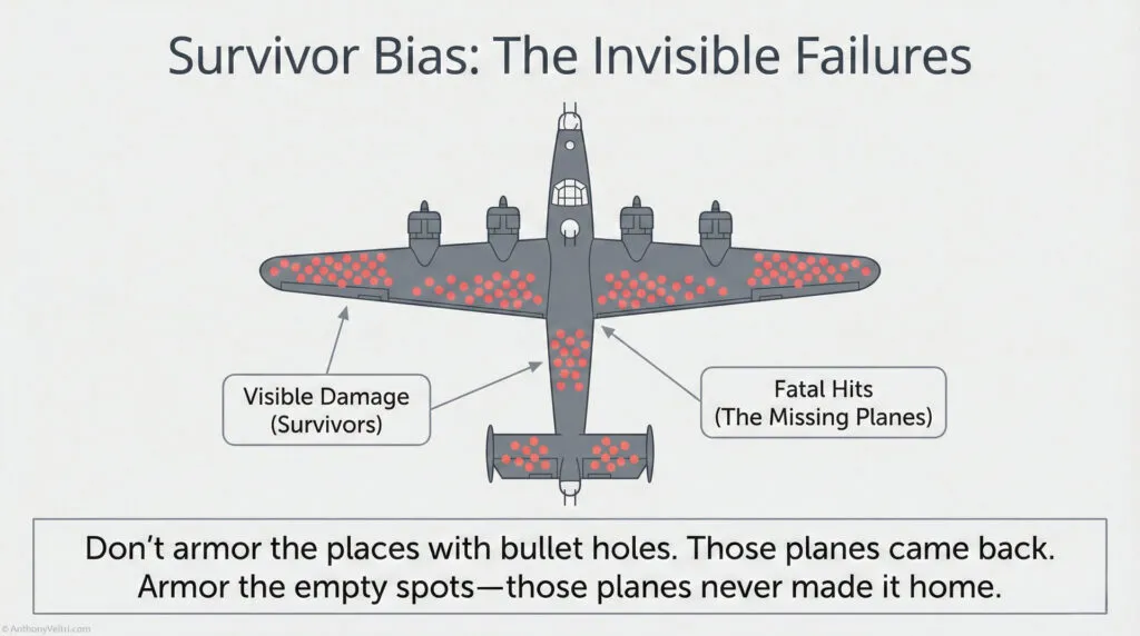
Classic example: During World War II, statistician Abraham Wald was asked to study where to add armor to bomber aircraft. The military showed him data on where returning planes had bullet holes. His recommendation: Don’t armor where the bullet holes are. Armor where the bullet holes AREN’T.
Why? Survivor bias. The planes you’re looking at are the ones that made it back. The bullet holes you see are in places where a plane can take damage and still fly. The places with NO bullet holes on returning planes are the critical areas (engines, cockpit, fuel tanks) because planes hit there didn’t make it back.
You’re only seeing the survivors. The failures are invisible.
The Crosswalk: #
| What You Say | Formal Term | Example |
|---|---|---|
| “Everyone who does this seems to succeed” | Survivor bias | Only seeing the winners, not the failures |
| “For every success story, how many tried and failed?” | Accounting for unseen cases | Denominator problem |
| “This worked for them, but how many tried?” | Base rate with full population | Need total attempts, not just successes |
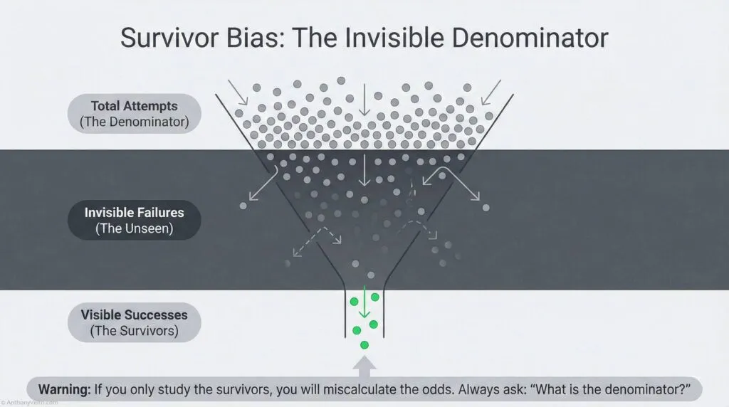
Working Rule – Always Ask About The Denominator
Whenever you hear a success story, ask how many tried.
Your real odds live in the whole population, not just the survivors in front of you.

Why This Matters for Base Rate Estimation: #
If you estimate base rates by looking only at success stories, you’ll be wildly overconfident.
Example: Building a Public Teaching Platform
You look at people who successfully built doctrine platforms (Simon Wardley, Paul Graham, Ribbonfarm authors). You see 5-10 people who succeeded. You think “If they can do it, I can too. Looks like high success rate.”
What you DON’T see: The 50-100 people who tried to build similar platforms and quit after 6 months when nobody read their content. The failures are invisible. They deleted their blogs, stopped posting, went back to regular jobs.
Real base rate might be:
- 100 people try to build teaching platforms
- 90 quit within a year
- 5-10 succeed
- P(success | attempt) = 5-10%
But if you only look at the survivors, you estimate P(success) = 100% because everyone you see succeeded.
How to Correct for Survivor Bias: #
1. Ask: “For every success I see, how many failures am I NOT seeing?”
Don’t just count successes. Estimate the denominator (total attempts).
2. Seek out failure stories.
Talk to people who tried and quit. Understand why they failed. This gives you the full distribution, not just the success tail.
3. Be skeptical of advice from successful people.
Successful people often attribute their success to their approach, ignoring luck and survivor bias. Their advice might be “do what I did” when the real answer is “do what I did AND get lucky.”
Why This Matters for Your Decisions: #
If you’re considering a high-risk path (building platform, starting business, career change), don’t just look at the people who succeeded. Look at the base rate of attempts, including failures.
Then ask: “What makes me different from the people who failed? Do I have advantages they didn’t (resources, skills, network, timing)? Or am I just optimistic?”
If you can’t identify specific advantages, assume you face the same base rate everyone else does. Don’t assume you’re special just because you want to be.
Section 11: Calibrated Confidence (Are You Right as Often as You Think?) #
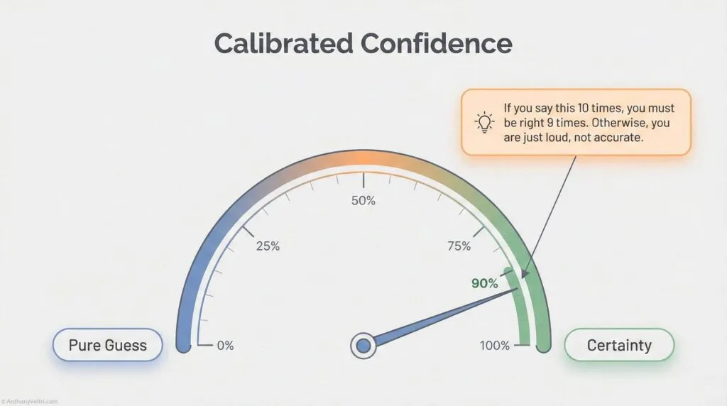
Most people are poorly calibrated.
When they say “90% confident,” they’re only right 70% of the time (overconfident).
When they say “50% confident,” they’re avoiding making a real estimate.
The formal term is “calibration.” It means your confidence level should match your actual accuracy rate. If you say “80% confident” 100 times, you should be right approximately 80 times.
The Crosswalk: #
| What You Say | What It Should Mean | What It Often Means (Poorly Calibrated) |
|---|---|---|
| “I’m 90% sure” | Right 9 out of 10 times | Right 7 out of 10 times (overconfident) |
| “I’m 50% sure” | Right half the time | “I don’t know” (avoiding estimate) |
| “I’m 99% sure” | Right 99 out of 100 times | Right 80 out of 100 times (very overconfident) |
| “I’m 70% confident” | Right 7 out of 10 times | Actual accuracy matches stated confidence |
How to Calibrate: #
1. Track your predictions.
Write down your estimates with confidence levels. “I’m 80% confident this integration will succeed.”
2. Check how often you’re actually right.
After 20 predictions at “80% confident,” count how many were correct.
3. Adjust your confidence language accordingly.
If you were right 12 out of 20 times (60% actual), you’re overconfident. When you feel “80% sure,” you should say “60% confident.”
If you were right 16 out of 20 times (80% actual), you’re well-calibrated. Keep using “80% confident” when you feel that level of certainty.
Why This Matters: #
Better calibrated estimates lead to better decisions.
If stakeholders can’t trust your confidence levels (you say “90% sure” but you’re only right 60% of the time), they’ll stop listening to your probability estimates. You’ll lose credibility.
If you’re well-calibrated (when you say “90% sure,” you’re right 90% of the time), stakeholders can use your estimates to make good decisions. They know what “90% confident” means coming from you.
Example from Incident Command: #
An incident commander says “80% confident we’ll have this contained by tomorrow.” Stakeholders need to know: Does that mean 80% or does it mean “I hope so but who knows”?
If the IC is well-calibrated (right 80% of the time when they say “80% confident”), stakeholders can trust that estimate and plan accordingly.
If the IC is poorly calibrated (only right 50% of the time when they say “80% confident”), stakeholders learn to ignore the confidence level and assume everything is 50-50. The IC has lost the ability to communicate probability effectively.
The Rule: #
Track your predictions. Check your accuracy. Recalibrate as needed. This is the only way to get good at estimating probabilities under uncertainty.
Douglas Hubbard (author of “How to Measure Anything”) teaches this as a core skill for decision-makers. Most people are overconfident. Calibration training can fix this.
Section 12: Value of Information (When Should You Gather More Data?) #
Common question: “Should we make a decision now, or gather more information first?”
The formal framework is “value of information.” It means you calculate:
- Cost of gathering information (time, money, opportunity cost)
- Expected value of information (how much better decision could you make with more data?)
- Compare: If value > cost, gather data. Otherwise, decide now.
The Crosswalk: #
| What You Say | Formal Term | Example |
|---|---|---|
| “We need more data before deciding” | High value of information | Decision threshold close, more data could change it |
| “We know enough, let’s decide” | Low value of information | Already 90% confident, more data won’t change decision |
| “This research isn’t worth the time” | Cost exceeds value | Delay costs more than potential wrong decision |
Working Rule – Only Buy Data That Can Change Your Mind
Extra analysis is only worth it if it might change the decision.
If you are already well past your decision threshold, decide.
Do not delay just to feel safer.
Example: Evacuation Decision #
- Current confidence: 60% hurricane will hit
- Threshold for evacuating: 70%
- Value of information: High (better forecast could push you over threshold and change decision)
- Cost of waiting: 6 hours for next forecast update
- Decision: Wait for better data if it’s safe to do so
vs.
- Current confidence: 90% hurricane will hit
- Already well over 70% threshold
- Value of information: Low (even if forecast updates to 80%, you’d still evacuate)
- Cost of waiting: 6 hours (roads get congested, harder to evacuate)
- Decision: Evacuate now, don’t wait for more data
Example: System Architecture Decision #
- Current confidence: 95% federated approach will work better than integrated approach
- Already very confident, more analysis unlikely to change decision
- Value of information: Low
- Cost of waiting: Delays project 2 months while you study it more
- Decision: Proceed with federated approach now
vs.
- Current confidence: 55% federated approach will work better (close call)
- Small amount of additional analysis could change your decision
- Value of information: High (might save you from wrong choice)
- Cost of waiting: 2 weeks for small pilot study
- Decision: Run pilot study, gather data, then decide
The Rule: #
Don’t gather information just because you can. Gather information when it’s likely to change your decision and the benefit of a better decision exceeds the cost of delay.
If you’re already confident (90%+ probability) and more data won’t change that, decide now. Don’t delay for perfect information that won’t affect the outcome.
If you’re uncertain (40-60% probability) and decision threshold is close, gather more data if the cost is reasonable. Better information could prevent a costly mistake.
Section 13: Ranges vs Point Estimates (Honest Uncertainty) #
You don’t need exact numbers. You need ranges that reduce uncertainty.
Douglas Hubbard’s key insight: Most people think “I can’t measure this precisely, so I won’t measure it at all.” Wrong. You should think “I don’t know exactly, but I’m 90% confident it’s between X and Y.”
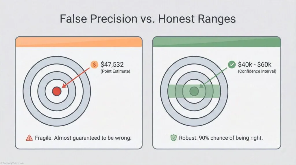
Ranges are better than point estimates because:
- More honest (acknowledge uncertainty)
- More useful (stakeholders know the spread)
- Easier to estimate (don’t need false precision)
- Better decisions (planning for range, not single point)
The Crosswalk: #
| What You Say | Formal Term | Why It’s Wrong/Right |
|---|---|---|
| “This will cost exactly $47,532” | Point estimate (false precision) | Wrong: You don’t actually know to the dollar |
| “This will cost between $40K and $60K” | Range estimate | Right: Honest about uncertainty |
| “90% confident it will cost $40K-$60K” | Confidence interval | Even better: Specifies confidence level |
Working Rule – Ranges Beat Fake Precision
It is better to give a range you are truly confident in than a single number you are not.
“Ninety percent sure it is between four and nine months” is honest.
“It will take six months” is pretend.
Why Ranges Are Better: #
Wrong (false precision): “We’ll have it contained in exactly 4.7 days.”
Nobody believes this. You don’t know to the nearest tenth of a day. You’re signaling overconfidence.
Right (honest uncertainty): “90% confident we’ll have it contained in 3 to 7 days, most likely around 5 days.”
This is more honest AND more useful. Stakeholders can plan for 3-7 day range, with 5 days as the central estimate. They know what uncertainty looks like.
How to Estimate Ranges: #
Step 1: Don’t think “what’s the exact number?” Think “what’s the range I’m 90% confident about?”
Step 2: Give lower bound and upper bound. “I’m 90% sure it’s between X and Y.”
Step 3: If you want, give a central estimate. “Most likely around Z, but could be as low as X or as high as Y.”
Example from Systems Integration: #
Wrong: “This integration will take exactly 6 months.”
Right: “90% confident this integration will take 4 to 9 months, most likely around 6 months.”
Stakeholders can now plan for 4-9 month range. If you deliver in 5 months, you’re a hero. If you deliver in 8 months, you’re still within stated range. If you take 10 months, you missed your estimate (only 10% of cases should fall outside the 90% range).
The Rule: #
Stop giving false precision. Give honest ranges with confidence levels.
If someone demands an exact number, push back: “I can give you a point estimate, but it’s false precision. The honest answer is a range. Which would you rather have, a precise number that’s probably wrong, or a range that’s probably right?”
Most stakeholders, once you explain it, prefer the range.
Section 14: The Technician to Executive Bayesian Crosswalk #
You’re already doing Bayesian reasoning. You just might not call it that.
Here’s the full vocabulary crosswalk:
| What You Say | Formal Term (Bayesian) | What Gordon Graham Calls It | Example |
|---|---|---|---|
| “What usually happens?” | Base rate | Starting point before High Risk/Low Frequency | “70% of integrations fail” |
| “I’ve seen this before, here’s what works” | Prior probability from experience | Recognition Primed Decision Making (RPDM) | “We tried this 10 times, 3 succeeded” |
| “We do this all the time, no problem” | High frequency, strong priors | High Frequency events (RPDM works) | “Daily operations, pattern is clear” |
| “We’ve never done this, hard to say” | Low frequency, weak priors | High Risk/Low Frequency (empty hard drive) | “Novel situation, no past pattern” |
| “Based on this new info, I’m more confident” | Bayesian updating | Learning as you go | “Was 30%, now 70% given new evidence” |
| “It depends on conditions” | Conditional probability | Context matters | “Success probability changes based on stakeholder buy-in” |
| “Even if unlikely, consequences too severe to risk” | Expected value, risk weighting | High Risk (study the consequences) | “Evacuate at 30% hurricane odds” |
| “I’m 80% confident” | Calibrated probability estimate | Honest uncertainty | “Right 8 out of 10 times when I say this” |
| “Between 4 and 9 months, most likely 6” | Range estimate with confidence | Honest about uncertainty | “90% confident it’s in this range” |
| “Everyone agrees, but same source” | Correlated evidence | Redundant information, not independent | “Three reports, one underlying source” |
| “We only tried once, hard to say” | Small sample size | Weak evidence | “Need more data points” |
| “For every success, how many failures?” | Survivor bias correction | The unseen failures | “Denominator problem” |
| “We rejected someone who could do the work” | False negative (Type II error) | Wrong evaluation format | “Panel interview filtered out capable person” |
| “What would prove me wrong?” | Seeking disconfirming evidence | Fighting confirmation bias | “Testing assumption, not defending it” |
| “Should we decide now or wait for more data?” | Value of information | Cost-benefit of gathering information | “Will more data change the decision?” |
Section 15: When to Use Each Tool #
Use RPDM (pattern matching, intuition) when:
- High frequency events (you do it all the time)
- Your hard drive is full (strong priors from experience)
- Time pressure (no time for analysis)
- Low stakes (consequences of being wrong are small)
Use Bayesian reasoning (slow down, think it through) when:
- Low frequency events (you don’t do this often)
- Your hard drive is empty (weak or no priors)
- Discretionary time (you CAN slow down)
- High stakes (consequences of being wrong are severe)
- Gordon Graham’s danger zone: High Risk, Low Frequency with Discretionary Time
Use pre-loaded systems/training when:
- Low frequency events (empty hard drive)
- No discretionary time (must act immediately)
- High stakes (can’t afford to think it through on the fly)
- Gordon Graham’s scary zone: High Risk, Low Frequency, Non-Discretionary Time
Section 16: Practical Checklist (Are You Thinking Bayesian-ly?) #
You’re doing Bayesian reasoning if you:
Foundation:
- ✅ Start with base rates (what usually happens)
- ✅ Update beliefs when new evidence arrives
- ✅ Think conditionally (“it depends on…”)
- ✅ Weight probability by consequences (expected value)
Avoiding Common Errors:
- ✅ Don’t ignore base rates (start with what usually happens)
- ✅ Seek disconfirming evidence (fight confirmation bias)
- ✅ Account for survivor bias (ask “how many tried and failed?”)
- ✅ Understand which errors cost more (false positive vs false negative)
Evaluating Evidence Strength:
- ✅ Check if evidence is independent or correlated
- ✅ Consider sample size (one data point vs many)
- ✅ Ask if more information would change your decision (value of information)
Expressing Uncertainty Honestly:
- ✅ Give ranges, not false precision (“4-9 months, most likely 6”)
- ✅ Express confidence levels (“80% confident”)
- ✅ Track predictions and recalibrate if needed
You’re NOT thinking Bayesian-ly if you:
- ❌ Think in binaries (“it will work” or “it won’t” with no probability)
- ❌ Ignore context (“this is always true” regardless of conditions)
- ❌ Don’t update beliefs (“I’ve always thought this” despite new evidence)
- ❌ Claim false certainty (“I’m 100% sure” when you can’t be)
- ❌ Ignore base rates (“I feel like it will work” despite 70% failure rate)
- ❌ Only seek confirming evidence (confirmation bias)
Section 17: Field Examples (Doctrine in Practice) #
Example 1: Incident Command (Wildland Fire) #
Situation: Fire is spreading. Incident commander needs to decide: evacuate nearby community or let residents shelter in place?
High Risk, Low Frequency: This IC hasn’t faced this exact scenario before (low frequency). Consequences of wrong decision are severe (lives at risk, high risk).
Bayesian approach:
Base rate: “In past fires with similar conditions (wind speed, fuel moisture, terrain), what percentage led to structure loss in nearby communities?”
- Look at records: 30% of similar fires reached structures
Conditional probability: “How do conditions today compare?”
- Wind is stronger than average: increases risk
- Fuel moisture is lower than average: increases risk
- Community has good defensible space: decreases risk
- Updated estimate: 40% chance fire reaches structures
Expected value: “What are consequences of each decision?”
- Evacuate unnecessarily: $50K cost, disruption, some risk during evacuation
- Don’t evacuate when fire reaches community: Lives at risk, $10M+ property loss
- Even at 40% probability, expected value strongly favors evacuation
Value of information: “Should we wait for better forecast?”
- Next weather update in 2 hours
- But evacuation takes 3 hours, and wind is picking up
- Cost of waiting exceeds value of better information
- Decide now: Evacuate
Decision: Evacuate based on 40% probability weighted by catastrophic consequences if wrong.
Outcome: Fire changes direction, doesn’t reach community. Evacuation was unnecessary (in hindsight). But decision was correct given information available at the time. Expected value justified evacuation even at 40% probability.
Example 2: System Integration (Federal Coalition) #
Situation: You’re asked to integrate five agency systems. Past similar integrations have 70% failure rate.
High Risk, Low Frequency: You haven’t integrated THIS particular set of agencies before (low frequency). Failure would cost $5M and set program back 18 months (high risk).
Bayesian approach:
Base rate: “What’s the success rate for similar integrations?”
- Past data: 30% succeed, 70% fail
- Prior estimate: 30% success probability
New evidence: “What’s different about this integration?”
- Evidence 1: Executive sponsor is committed (past integrations with exec sponsor: 50% success)
- Evidence 2: Three of five agencies have named stewards (integrations with stewards: 60% success)
- Evidence 3: Stakeholders have actually signed MOU (not just verbal commitment): 70% success with signed agreements
Bayesian updating:
- Start: 30% (base rate)
- After exec sponsor evidence: Update to 50%
- After named stewards evidence: Update to 60%
- After signed MOU evidence: Update to 70%
- Posterior estimate: 70% success probability
Expected value:
- P(success) = 70%, value = $10M benefit
- P(failure) = 30%, cost = $5M loss
- Expected value = (0.7 × $10M) – (0.3 × $5M) = $7M – $1.5M = $5.5M positive
Value of information: “Should we do a pilot first?”
- Pilot would cost $500K and 3 months
- Would give us better estimate (maybe update from 70% to 80% or down to 60%)
- Decision threshold: We’d proceed if >50% probability
- Already at 70%, well above threshold
- Pilot unlikely to change decision (would have to drop below 50% to change course)
- Value of information: Low
- Decision: Proceed with full integration without pilot
Outcome: Integration succeeds (as predicted 70% probability). If it had failed (30% chance), decision would still have been correct given information available.
Example 3: Career Decision (Building Public Platform) #
Situation: You’re considering leaving stable contractor job to build public teaching platform (doctrine guides, video content, consulting).
High Risk, Low Frequency: You haven’t done this before (low frequency). If it fails, you’ve lost income and time (high risk for you personally).
Bayesian approach:
Base rate with survivor bias correction: “How many people try to build teaching platforms? How many succeed?”
- Visible successes: You can name 5-10 people who built successful platforms
- Hidden failures: Estimate 50-100 tried and quit
- Base rate: 5-10 successes out of 100 attempts = 5-10% success rate
- Prior estimate: 5-10% you’ll succeed
New evidence: “What advantages do you have?”
- Evidence 1: You have 20 years field experience (real credential, not just theory)
- Evidence 2: You can produce professional video (differentiated capability)
- Evidence 3: You already have some content (not starting from zero)
- Evidence 4: You have network that can distribute (warm intros, not cold audience building)
Conditional probability: “Do these advantages significantly change the odds?”
- Most failures: People with theory but no field experience (you have field experience)
- Most failures: People who can’t produce professional content (you have production capability)
- Most failures: People starting from scratch (you have initial content + network)
- Updated estimate: Maybe 30-40% success probability (still not great, but better than base rate)
Expected value: “What are consequences?”
- P(success) = 35%, value = $100K+/year income + meaningful work + autonomy
- P(failure) = 65%, cost = Lost 1-2 years + back to contractor work at similar pay
- Expected value: Harder to quantify, but depends on how much you value autonomy/meaningful work vs income stability
Value of information: “Should you build more before deciding?”
- Could create content for 6 months while staying employed, see if it gets traction
- Cost: 6 months part-time effort
- Value: Reduces uncertainty (if no one engages with content, probability drops; if people engage, probability rises)
- High value of information (could change decision from 35% to either 60% or 15%)
- Decision: Build platform part-time for 6 months, gather data, then decide whether to commit full-time
This is Bayesian reasoning for career decisions:
- Start with base rate (survivor bias corrected)
- Identify specific advantages that might change odds
- Update probability estimate
- Calculate expected value (including non-financial value)
- Assess value of information (pilot test before full commitment)
- Make decision based on updated probability, not base rate alone
Section 18: Why This Matters for Forward-Deployed Work #
Field environments have high uncertainty, incomplete information, and time pressure. Bayesian thinking helps you make better decisions in these conditions.
Gordon Graham’s framework: Most mistakes happen on high-risk, low-frequency events. Your hard drive is empty (no strong patterns from experience). If you have discretionary time, slow down and think it through. If you don’t have discretionary time, you need pre-loaded systems and training.
Bayesian reasoning is what “slow down and think it through” looks like in practice:
- Check base rates (what usually happens in situations like this)
- Gather evidence (what’s specific about this case)
- Update probability (Bayesian revision based on evidence)
- Weight by consequences (expected value, not just probability)
- Assess value of information (should I decide now or gather more data?)
- Make decision (act on updated probability, acknowledge uncertainty)
When you don’t have time to think it through (high risk, low frequency, no discretionary time), you need different approach:
- Pre-loaded procedures (fire service calls them SOPs, Military examples could include Immediate Action Drills, in aviation it could be abnormal procedures checklist or memory items)
- Training that simulates high-risk scenarios
- Systems that reduce decision load in crisis
- Named stewards who own critical processes
Bayesian thinking doesn’t replace training and systems. It complements them.
Use training/systems for non-discretionary time events. Use Bayesian reasoning for discretionary time events.
Section 19: How to Get Started #
Step 1: Track one decision this week.
Pick a decision where you estimated probability. Write down:
- Your estimate (“70% confident this will work”)
- Your reasoning (base rate, evidence, updating process)
- The outcome (did it actually work?)
Step 2: After a month, check your calibration.
Count how many times you were right when you said “70% confident.” If you’re right 7 out of 10 times, you’re well-calibrated. If you’re right 4 out of 10 times, you’re overconfident. Recalibrate.
Step 3: Practice the base rate question.
Every time someone asks you to estimate something, ask yourself first: “What usually happens in situations like this?” Don’t skip to specific details. Start with the base rate.
Step 4: Use the 2×2 matrix.
For any decision, ask: Is this high or low risk? Is this high or low frequency? If you’re in the high-risk, low-frequency box with discretionary time, slow down. Use Bayesian reasoning.
Step 5: Seek disconfirming evidence.
Next time you have a strong belief about something, force yourself to articulate the best case AGAINST your position. What evidence would prove you wrong? Go look for that evidence specifically.
That’s it. You’re now doing Bayesian reasoning intentionally instead of just intuitively.
Over time, this becomes automatic. You’ll catch yourself checking base rates, updating on evidence, thinking conditionally, weighting by consequences. The vocabulary becomes natural.
You don’t need to be a statistician. You don’t need to know the math. You just need to recognize the patterns in how you already think, and give yourself permission to be explicit about uncertainty instead of pretending to have certainty you don’t actually have.
Further Resources #
Books:
- Douglas Hubbard, “How to Measure Anything” (Bayesian reasoning for business decisions, calibration training, value of information)
- Nate Silver, “The Signal and the Noise” (Bayesian thinking in forecasting, avoiding overconfidence)
Videos:
- Gordon Graham, “High Risk/Low Frequency Events” (fire service/public safety perspective, RPDM vs Bayesian reasoning)
- https://www.youtube.com/watch?v=Og9Usv82CdU
Training:
- Calibration exercises (Hubbard’s work teaches this systematically)
- Track your predictions, check your accuracy, recalibrate
Remember:
- Most of what you do goes right (RPDM handles high-frequency events)
- Mistakes happen on high-risk, low-frequency events (empty hard drive)
- Slow down when you have discretionary time (use Bayesian reasoning)
- This is vocabulary for thinking you already do (recognition, not education)
A Note on This Guide #
This guide draws from multiple sources: Reverend Thomas Bayes (1763 mathematical foundation), Gordon Graham (fire service risk management), Douglas Hubbard (measurement under uncertainty), and decades of practitioner experience in high-consequence environments.
The Bayesian framework isn’t new. The crosswalk to practitioner language is what makes it usable.
If you found this useful, you’re probably already thinking this way. You just didn’t have words for it. Now you do.
Use them.
(Here Be Dragons) #
#
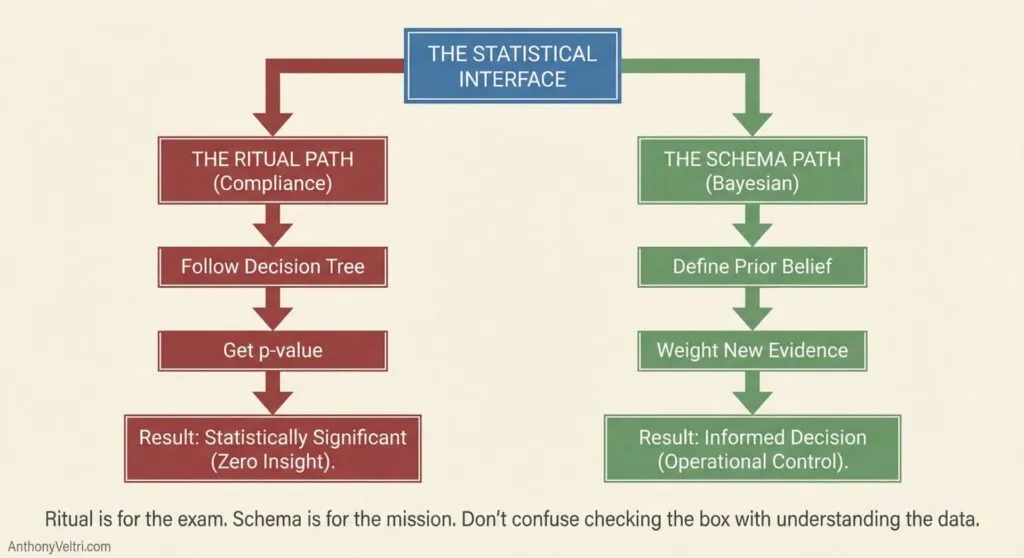
Before we get to the visuals nobody showed you, let’s talk about why you probably hated statistics class. It wasn’t because you’re bad at math. It was because you were taught Ritual without Schema.
A Schema is a mental template that tells you what something means and why it happens in a specific sequence (like the steps of ordering at a restaurant). Statistics is often taught as pure ritual: “If p > 0.05, look at this row; if p < 0.05, look at that row. Do not ask why. Just memorize the steps for the exam”.
This is Governance Theater applied to mathematics. You can follow the steps perfectly and have zero understanding of the data. You can have perfect compliance while completely missing competence.
Traditional statistics optimizes for what is easy to grade (picking the right option from a decision tree). This doctrine optimizes for what actually matters: making good decisions under uncertainty.
Bayesian thinking isn’t about following a ritual; it’s about asking: “Given this evidence, what should I believe, and what should I do?”. That is a schema question.
Now, let’s look at what p-values and z-values actually measure, and why the visuals matter.
The Picture They Never Drew #
If you’re over 40 and took stats in grad school, you saw p-values as numbers on a page. p = 0.04. p = 0.002. Maybe you looked them up in a table at the back of the textbook.
Nobody showed you the picture.
Most stats courses jump straight to “here’s the formula, look up the critical value” without showing you what’s actually happening geometrically. You memorized that p < 0.05 means “statistically significant” without ever seeing what that 0.05 represents spatially.
This section fixes that. Not because you need p-values for the Bayesian framework in this guide (you don’t), but because understanding what p-values measure makes it clearer why Bayesian reasoning asks a better question.
What p-values Actually Look Like #
When you run a statistical test, you’re asking: “If there’s really no effect (the null hypothesis), how surprising would it be to see data this extreme?”
(Note for the statistical purists: by “surprising,” we technically mean “improbable under the assumed model,” but for operational decision-making, “surprise” is the useful intuition.)
The ‘Null’ = The Nothing Burger Before looking at the curve, you have to define the “Null Hypothesis.” In plain English, this is the Boring Default.
- In a drug trial, the Null is: “This pill does nothing.”
- In a marketing test, the Null is: “This new button didn’t change conversion rates.”
- In operations, the Null is: “This is just normal random variation.”
Statistical tests always start by assuming the Boring Default is true. They don’t prove the new thing works; they just check if the data is so weird that the Boring Default looks ridiculous.
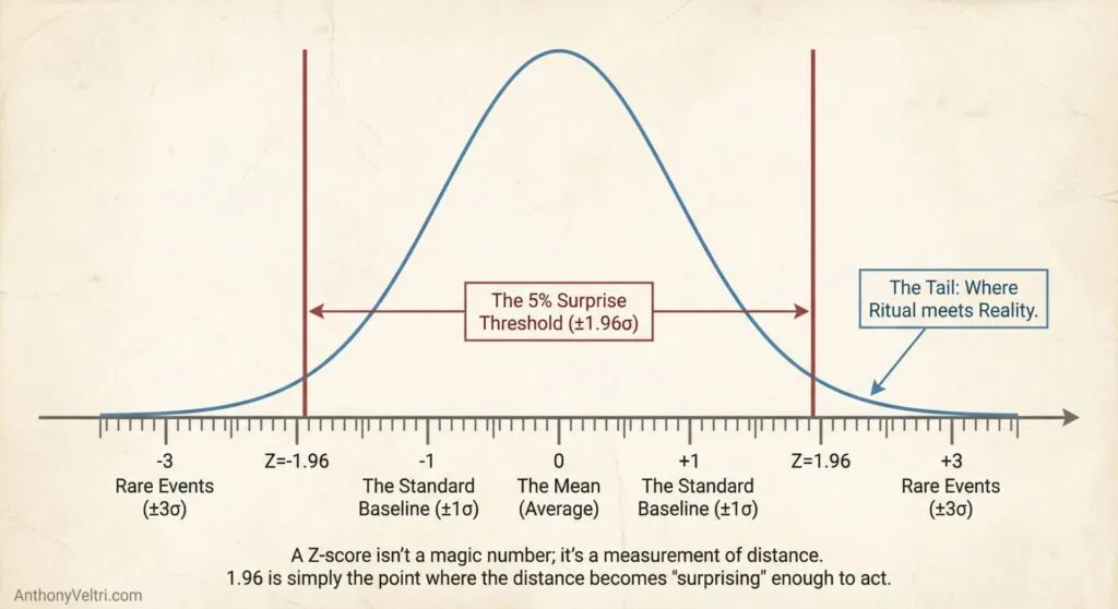
Think of a bell curve centered at zero. That’s your null hypothesis. No effect. No difference. Nothing happening.
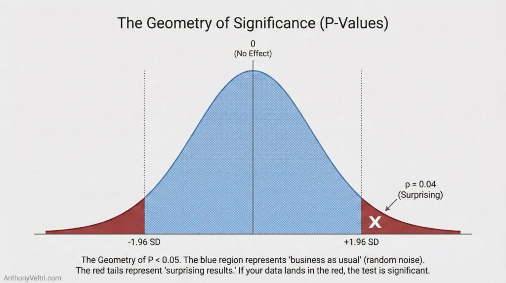
The middle 95% of that curve represents ordinary results you’d expect from random noise. The outer 5% (split between both tails, 2.5% on each side) represents surprising results. Results you’d only see 5% of the time if the null hypothesis were actually true.
When someone says p < 0.05, they’re saying their observed result landed out in one of those tail regions. Far enough from the center (about 2 standard deviations out) that Fisher decided it was “surprising enough to investigate.”
That’s the entire basis for the magic threshold. If you’d only see data this extreme 5% of the time when nothing’s happening, maybe something actually is happening.
The Dictionary of Belief #
Before the example, let’s translate the three key terms.
- The Prior (The Anchor): What you believed before you saw the new data. This is your Base Rate or “going in” assumption. (e.g., “Integrations usually fail.”)
- The Likelihood (The Tug): The new evidence you just collected. The stronger the evidence (more data points), the harder it pulls. (e.g., “This specific pilot worked 70% of the time.”)
- The Posterior (The Balance Point): Your new belief. It is the compromise between your Anchor and the Tug.
The Mechanism: If your Prior is weak (“I have no idea”) and the Evidence is strong (“I ran 1,000 tests”), the Posterior shifts entirely to the Evidence. If your Prior is strong (“Gravity exists”) and the Evidence is weak (“My pencil floated for a second”), the Posterior barely moves. The Anchor holds.
The Standard Deviation Version #
Different p-value thresholds map to specific distances from the center:
- 1.96 standard deviations from zero = p < 0.05 (Fisher’s classic threshold)
- 2.58 standard deviations from zero = p < 0.01 (More stringent)
- 3.0 standard deviations from zero = p < 0.003 (Very stringent)
- 5.0 standard deviations from zero = p < 0.0000003 (What particle physics uses)
Different fields pick different thresholds based on what false positives cost. Physics uses 5-sigma because they can’t afford to announce a new particle that doesn’t exist. Social science historically used 2-sigma (p < 0.05) because Fisher suggested it in 1925 and it stuck.
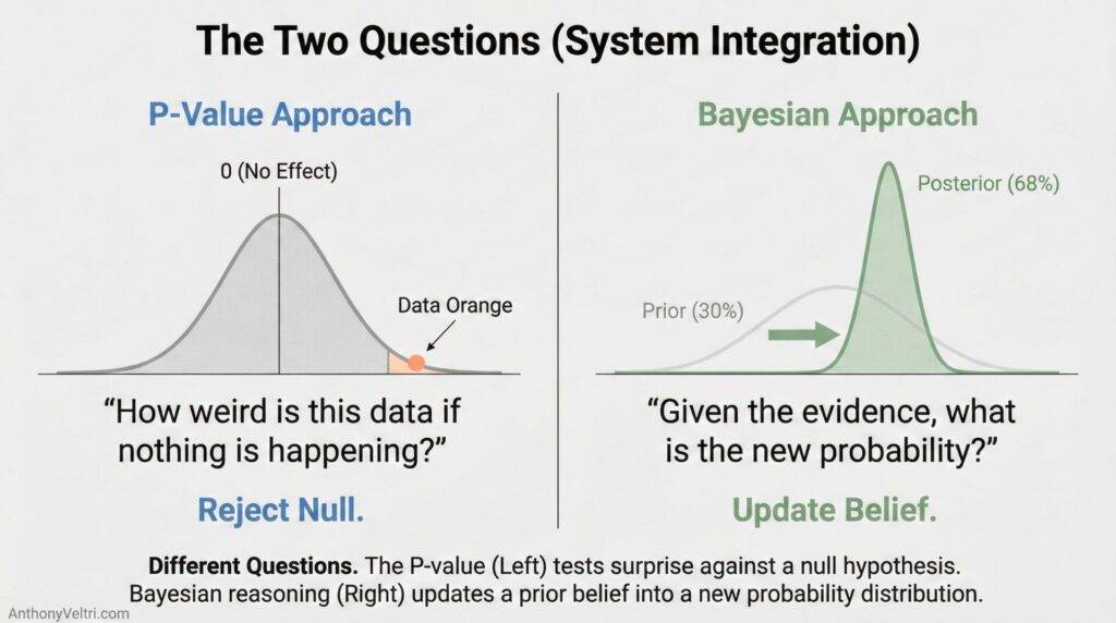
Example 1: System Integration #
You’re evaluating whether adding a named steward actually improves integration success rates.
Frequentist approach (p-values):
You run 50 integrations. 25 with named stewards, 25 without. Success rates: 70% with steward, 50% without. You run a statistical test and get p = 0.04.
What this tells you: “If stewards made no difference (the null), I’d only see a 20 percentage point gap this large or larger about 4% of the time. That’s rare enough to be surprising.”
What it doesn’t tell you: The probability that stewards actually help. The size of the effect. Whether a 20-point improvement matters operationally.
Bayesian approach (what this guide teaches):
- Start with base rate: Past integrations succeed 30% of the time (no steward).
- Evidence arrives: In this sample, integrations with named stewards succeeded 70% of the time.
- Update estimate: “I’m now 85% confident that integrations with named stewards succeed between 55% and 80% of the time, with most likely value around 68%.”
This directly answers the question you actually care about: “What do I now believe about steward effectiveness, given this evidence?” Not “How surprising is this data if stewards don’t help?”
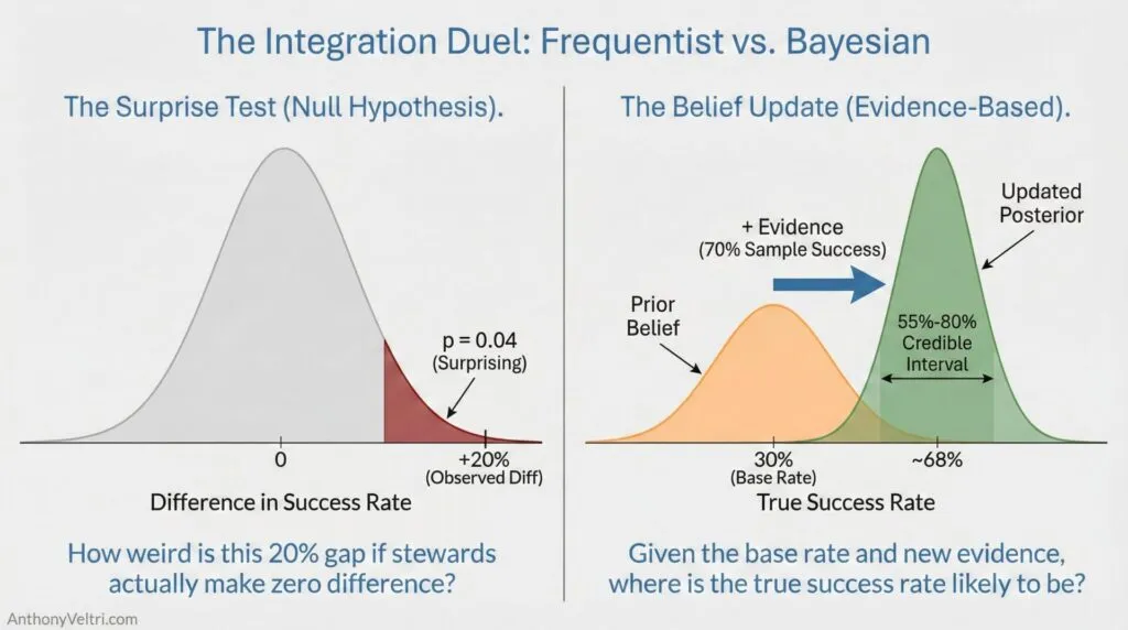
| Feature | The P-Value Approach | The Bayesian Approach |
| The Question | “How weird is this data if nothing is happening?” | “Given this data, what is likely happening?” |
| The Output | A yes/no flag (Significance) | A probability estimate (Confidence) |
| Prior Knowledge | Ignored (Assumes blank slate) | Essential (Starts with Base Rates) |
| Best Used For | Quality Control, Science Experiments | Operational Decisions, Betting, Strategy |
Example 2: Fire Containment and Weather #
Incident commander needs to decide whether to evacuate based on forecast wind speed increase.
Frequentist approach (p-values):
Weather model shows wind speed increasing 15 mph over baseline. Historical data shows wind increases of 15+ mph only happen 3% of the time under current conditions. p = 0.03.
What this tells you: “If conditions were normal, I’d only see wind increases this large 3% of the time. This is surprising.”
What it doesn’t tell you: Probability that the forecast is accurate. Probability that fire reaches structures. What evacuation decision to make.
Bayesian approach (what this guide teaches):
- Base rate: Under similar conditions historically, 40% of fires reach nearby structures when wind increases.
- Current evidence: Wind forecast shows 15 mph increase (strong evidence). Fuel moisture is lower than usual (increases risk). Community has good defensible space (decreases risk).
- Updated estimate: “Given all evidence, I estimate 55% probability fire reaches structures. Even at 55%, expected value strongly favors evacuation because consequence of being wrong is catastrophic.”
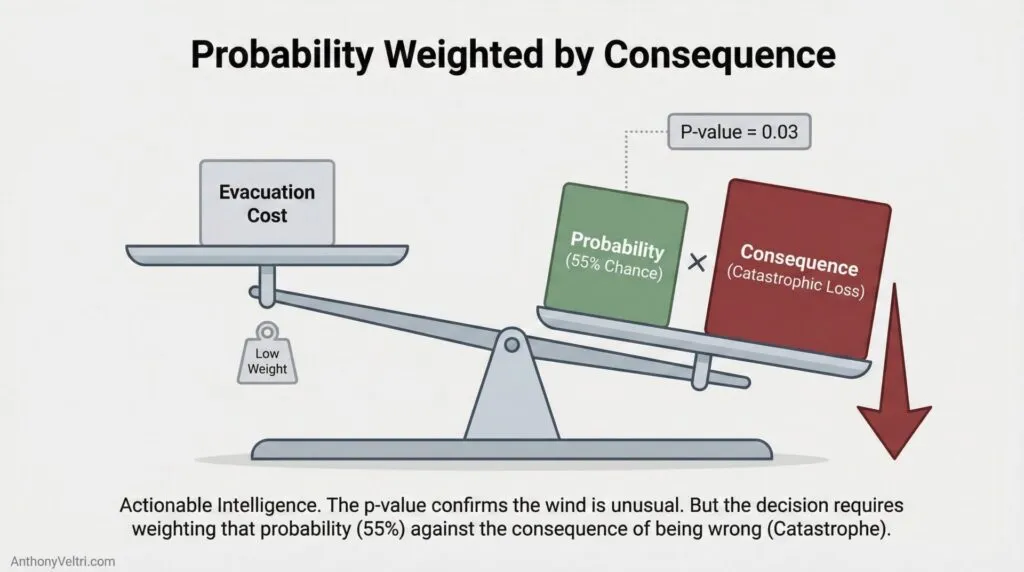
This framework gives you probabilities you can act on, weighted by consequences. The p-value just tells you the wind increase is statistically unusual.
Why Bayesian Reasoning Asks A Better Question #
Notice the difference:
- P-value asks: “How weird is this data if nothing’s happening?”
- Bayesian framework asks: “Given this data, what’s the probability distribution of what’s actually happening?”
Same visual intuition (bell curves, standard deviations, tail areas). Completely different question.
The Bayesian approach updates beliefs with evidence and gives you probability estimates you can use for decisions. The p-value approach gives you a yes/no flag based on whether you landed in a tail region of a hypothetical distribution.
For high-risk, low-frequency decisions (where this guide lives), you need the probability estimate and the consequence weighting. The p < 0.05 flag doesn’t get you there.
Working Rule: Know What Question You’re Answering #
When someone asks “Is it significant?”, they are often using a dangerous shorthand.
The Academic Trap (The “Health Check”):
In many circles disconnected from ground truth, “significance” is treated like a biological marker—like a cholesterol score or blood pressure reading.”Oh, p < 0.05? Great, we’re under the limit. The patient is healthy. The analysis is ‘good.’ The data is valid.”
This is a dangerous leap. A p-value is not a quality score. It is just a math output. It is entirely possible to have a “significant” p-value from irrelevant data, just as it is possible to have normal blood pressure while bleeding internally.
The Operational Reality:
When a decision-maker asks “Is it significant?”, they usually mean “Should we act on this?”
- P-values only tell you if the data is surprising under a null hypothesis.
- Bayesian reasoning tells you what to believe given the evidence.
For operational decisions, you need the second answer. Don’t confuse a math output for a clean bill of health.
The Bottom Line #
You don’t need to pick sides in the frequentist versus Bayesian philosophical war (which is still actively raging in statistics journals). You just need to recognize what each approach measures and use the thinking pattern that answers the question you’re actually asking.
If you’re making high-consequence decisions under uncertainty, you want probability estimates you can update as evidence arrives, weighted by what it costs to be wrong. That’s Bayesian reasoning. The p-value framework was built for something else (quality control, detecting manufacturing defects, agricultural experiments where you repeat trials many times).
Both approaches use the same visual geometry (distributions, standard deviations, tail probabilities). The Bayesian version just orients that geometry toward the questions operators actually need answered.
Why Your Brain Already Speaks Bayesian (AKA Z-Values, the distance nobody explained)
Statistics class taught you Ritual: “If Z > 1.96, report significance.” You passed the test, but you lacked the Schema.
P-values got the lookup table treatment. Z-values got the same.
“Find your z-score in the table. If z > 1.96, it’s significant at the 0.05 level.”
Nobody explained what z actually measures. Here’s the schema:
Z-Value = Standardized Distance From Center #
A z-value tells you: How many standard deviations away from the mean is this observation?
That’s it. It’s just distance, measured in standardized units.
This doctrine provides the missing visuals. A Z-score is simply a Standardized Ruler that measures how far an observation has strayed from the center.
Example That Makes It Concrete:
Average height: 5’8″ (68 inches) Standard deviation: 3 inches
Someone who is 6’2″ (74 inches):
- Raw difference: 74 – 68 = 6 inches taller than average
- Z-score: 6 / 3 = z = 2.0
- Meaning: “Two standard deviations above average height”
Someone who is 6’5″ (77 inches):
- Raw difference: 77 – 68 = 9 inches taller
- Z-score: 9 / 3 = z = 3.0
- Meaning: “Three standard deviations above average – extremely tall”
Why Standardized Units Matter:
Raw numbers don’t tell you much without context:
- “4.3 unit increase” – Is that big? Depends on what you’re measuring.
- “z = 2.0” – That’s always big, regardless of what you’re measuring.
Z-scores let you compare across different scales. A z-score of 2.0 means “unusually high” whether you’re measuring height, test scores, cancer biomarkers, or integration success rates.
The Table You Memorized #
The z-table converts between:
- Distance from center (z-score)
- Probability of being that far out or further (p-value area in tail)
Common values you (may have) memorized without understanding (I’m guilty of this too):
| Z-Score | Area in Tail | What It Means |
|---|---|---|
| 1.96 | 0.025 (2.5%) | Fisher’s 0.05 threshold (both tails = 5%) |
| 2.58 | 0.005 (0.5%) | More stringent (both tails = 1%) |
| 3.00 | 0.0013 (0.13%) | Very rare |
You looked these up in a table. Nobody showed you the curve. Nobody explained: “You’re just measuring how far out in the tail you landed, then converting that distance to a probability.”
Why The Schema Matters #
Ritual version: “Look up z in table. If z > 1.96, reject null hypothesis.”
You memorize. You pass the test. You have no idea what’s happening.
Schema version: “Your observation landed 2 standard deviations from the center. That’s far enough out that you’d only see this 5% of the time if nothing were happening. That’s rare enough to be surprising.”
Same math. Completely different understanding.
The Bayesian framework uses the same geometry (distributions, standard deviations, tail areas) but asks: “Given this evidence, what should I believe is happening?” not “How surprising is this if nothing is happening?”

More importantly, this framework gives you Labels for how you already think. When you walk into a restaurant and change your mind about the food because the table is sticky, you are doing Bayesian Updating. When a fire chief watches the wind pick up and adjusts their resource plan, they are using Conditional Probability.
You don’t need a new way to think. You need the Vocabulary to control the thinking you are already doing.
Field notes and examples #
- Field Note: Loosely Coupled Power Grabs
- Regime Recognition and the Cost of Asymmetric Errors: When Post-Hoc Learning Beats Theory-First
- Field Note: Handbook vs Terrain – When Constraint Forecasting Failed and Indications Won
- The Loudest Listener: When Interviews Become Something Else
- Field Note: The Symbol Is Not the Signal
- The Audition Trap: Why Panel Interviews Create False Negatives in Hiring
- Field Notes: What The Katrina Book Was Really For
Last Updated on February 22, 2026