Model vs. Terrain: Bridging the Interface Void on the Merritt Parkway
Ground Truthing Wireless Coverage Through CW Drive Testing
Before the Models: Where This Started
My grandfather was a licensed amateur radio operator. His callsign was W1EIG. I still have his license plate with that callsign on it.
He served as a B-24 crewman during the Second World War and came home with the kind of technical intuition that war sometimes produces in people who pay close attention to how things work and what happens when they do not. I know there was something else, a technical assignment connected to Japan after the surrender, something that required being dropped in and reporting back. The details were never fully explained to me. But he came home understanding that the ability to communicate when other systems failed was not a hobby. It was infrastructure.
He taught me photography. He taught me Morse code from a phonograph record, a training program that my brain clicked around in a way that earlier methods had not. He drove me to the examination sites when I tested for my Technician license and then the code endorsement, I was in seventh or eighth grade. And he helped me build a crystal radio from components we sourced not from Radio Shack but from an actual radio supply store that still sold tubes.
He also petitioned the Governor of Rhode Island to allow amateur radio operators to use their callsigns as vanity license plates. He got it done. There is a letter from the governor somewhere in my parents’ house. W1EIG on a Rhode Island plate. That is the kind of person he was.
What he gave me was a physical understanding of radio that started before I had any theoretical framework for it. Signal either reaches or it does not. The antenna is either properly matched or it is not. The connector is either clean or your whole day is compromised. You learn that with your hands before you learn it from a textbook, or you spend years unlearning the abstraction later.
The Gap I Did Not Know I Had
That foundation got me to analog RF, to HF and VHF communications, to a basic but honest understanding of propagation and path loss. What I did not have, until Katrina made it unavoidable, was the bridge between the physical RF layer and the network layer sitting on top of it.
On the Gulf Coast in 2005, I was immersed for the first time in the digital side of RF at operational scale. Not voice. Data. And I recognized quickly that I did not fully understand the gap between signal behavior and network behavior. Packet loss and signal loss were visibly the same problem expressed in two different vocabularies. Latency was not an abstract network metric. It was physics. The OSI model was not a diagram. It was a chain of physical constraints that each layer inherited from the one below it.
That gap sent me deeper. From HF analog into spread spectrum, frequency hopping, OFDM, pilot carrier signaling. CWNA certification. WiMAX. The RF propagation modeling work that followed, including the Merritt Parkway project described in this field note, was the place where those threads came together in a form I could apply. GIS as a vehicle for raster propagation modeling. Bare earth and canopy data folded into path loss calculations depending on the frequency being analyzed. The same spatial reasoning I had applied to beetle kill and crop stress and footprint detection showing up again in a completely different physical domain.
The convolution kernel does not care whether it is analyzing a forest canopy or an RF signal path. The physics changes. The reasoning pattern does not.
My grandfather understood that before I was born. He just expressed it in Morse code at five words per minute on a phonograph record in a living room in Rhode Island.
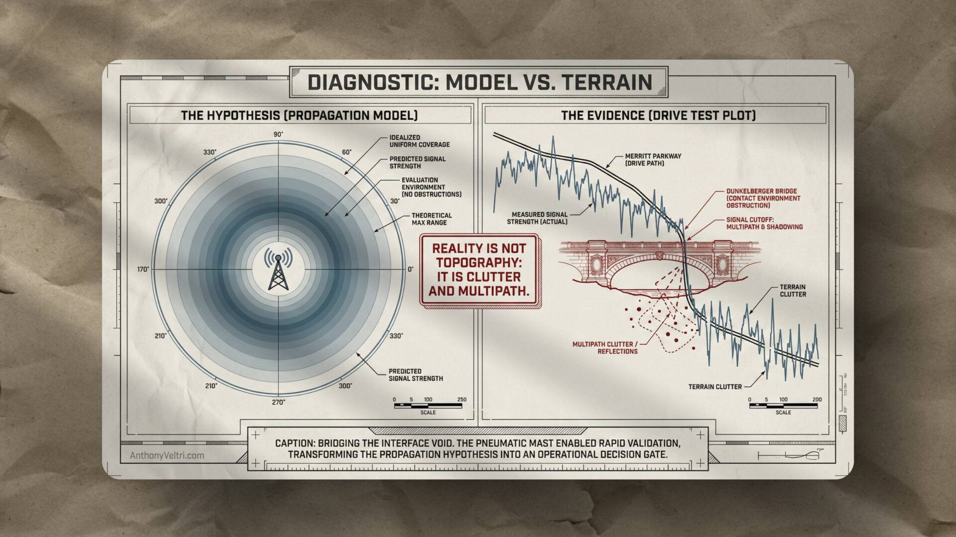
The Contact Event: Reality vs. The Propagation Model
Between late 2005 and early 2007, I was pulled into a problem that felt immediately familiar (wireless coverage modeling is not the same thing as wireless coverage reality).
RF engineers had already built propagation models for a distributed antenna system (DAS) along the Merritt Parkway corridor in Connecticut. However, installing hardware based only on a model is how you burn a budget. In wildland fire work, I learned the discipline: model first, then ground truth, then commit.
The ground truth here was CW (Continuous Wave) drive testing. This was the technical equivalent of the “can you hear me now” commercials of that era. We transmitted a steady signal and mapped where it actually reached. This was not about making prettier maps. It was about making a decision with confidence before mounting a single bracket.
The Constraint: Aesthetics, Architecture, and The Road Builder
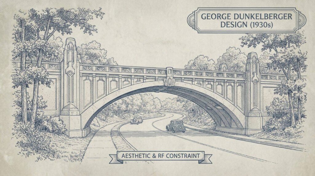
The Merritt Parkway is not a typical highway. It is a National Historic Landmark defined by a specific (and restrictive) aesthetic.
The history of the parkway is one of eminent domain and singular vision. While Robert Moses was famously carving parkways through New York with an iron hand, Connecticut was building the Merritt as a “Queen of Parkways” (intended exclusively for non-commercial vehicles).
This meant that the standard infrastructure of the wireless world (150-foot steel lattices) was legally and aesthetically impossible. The architectural soul of the parkway lives in its sixty-nine unique bridges designed by George L. Dunkelberger. No two bridges are identical. Some are Art Deco, others are Neo-Gothic, and all of them act as massive RF shields.
The situation: lots of proposed sites, modest heights, expensive mistakes
This was not classic “one tower, one test, done” work. A distributed antenna system means many proposed sites, lower antenna heights, and a ton of setup and teardown.
The standard approach was to rent a bucket truck (or crane) to raise a test antenna at each location. That works, but it is slow and bulky when you have dozens of candidate sites to validate.
That is where the bottleneck was: not driving, not math, not RF theory. Logistics.
My role: transmit-site operator, not the drive crew
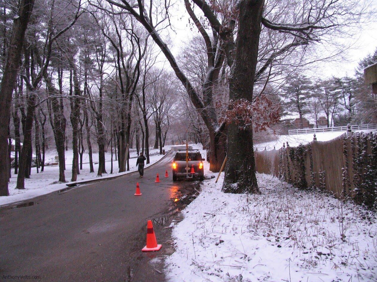
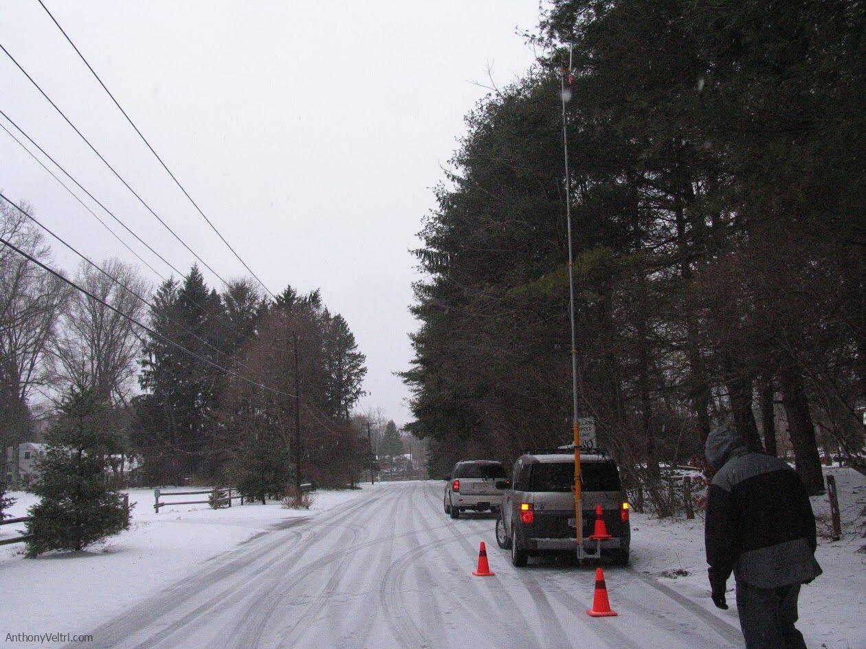
I was the transmit-site operator. I stayed at the proposed site, managed the mast and antenna, ran the transmitter, and kept the setup consistent from site to site.
A separate measurement vehicle did the drive testing. They were the ones dealing with route selection, GPS logging, and the reality of traffic.
That separation mattered, because at first I only knew “they have to drive slow.” Later I understood why it took them so long to cover a stretch of road.
They were not just driving slow. They had to drive at a specific speed band to keep the sampling valid. Slow enough to meet the sampling requirements and average out fast fading, but not so slow that the workflow collapsed or became unsafe in traffic.
Stage 2: The Revelation (Learning from the Navy Chief)
I came into this work with theory and RF propagation models. What I lacked was the operator’s knowledge of what breaks in the dirt.
On the Gulf Coast, I worked with a recently retired Navy Chief who lived in both worlds (he was equal parts theoretical engineer and hands-on operator). This was my Stage 2 Revelation. He showed me that my academic “Ritual” was vulnerable to variables I hadn’t considered.
He knew the math of path loss, but he also knew that a dirty coax connector or a poorly threaded terminator would corrupt an entire day’s dataset. He taught me that backup cables are not optional and that “what should be” is irrelevant if your hardware isn’t calibrated. He moved me from the “safety” of the model into the “friction” of the field. I am still grateful for that education. It is the difference between knowing RF theory and knowing how to produce decision-grade data.
The core pattern: hypothesis, evidence, commitment
The pattern was the same one I used in wildfire modeling:
- Model the invisible: propagation, path loss, terrain and clutter assumptions.
- Treat the model as a hypothesis: a starting point, not an answer.
- Ground truth fast: collect real measurements under controlled conditions.
- Commit with confidence: install only after you know the site earns it.
The win was not “more data.” The win was reducing the time between “candidate site” and “confident decision.”
The innovation: a five-minute mast deployment
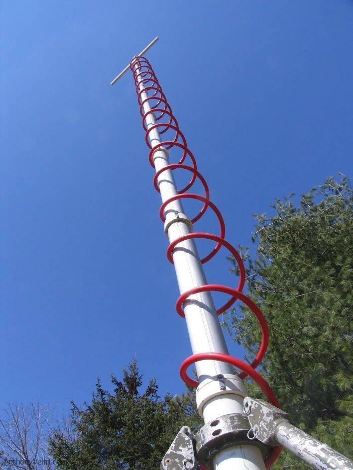
A contractor I met noticed I already had pneumatic masts for RF communications on my mobile mapping unit. He basically said, “That is a faster way to get a test antenna 30 to 40 feet up than bringing a bucket truck to every location.”
So I fitted a pneumatic mast to the back of my Honda Element. I could fold it down to drive, roll up to a proposed site, and be ready to transmit in about five minutes.
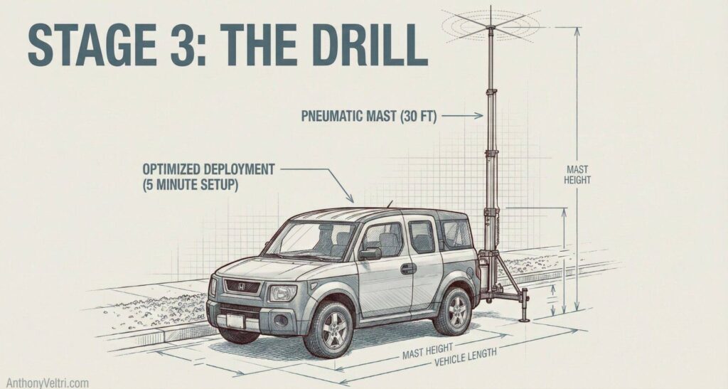
That changed the math. In very long days, we could validate roughly 15 sites per day. That speed came from geometry, not just equipment. A 150-foot cell tower has substantial range and requires extensive drive testing across a dense road network. A 30-foot pole-mounted antenna has limited reach, and the drive test completes quickly.
The pneumatic mast was optimized for this work: fast deployment, easy parking in neighborhood streets, and quick repositioning between sites. A bucket truck trying to validate 30 low-height sites would have burned days just on positioning and setup. It was like finding a parking spot with your Honda Civic in the city versus trying to park an extended cab King Ranch lifted dually. More optimized for the particular work.
Consistency beats perfection: antennas, coax, and controlled variables
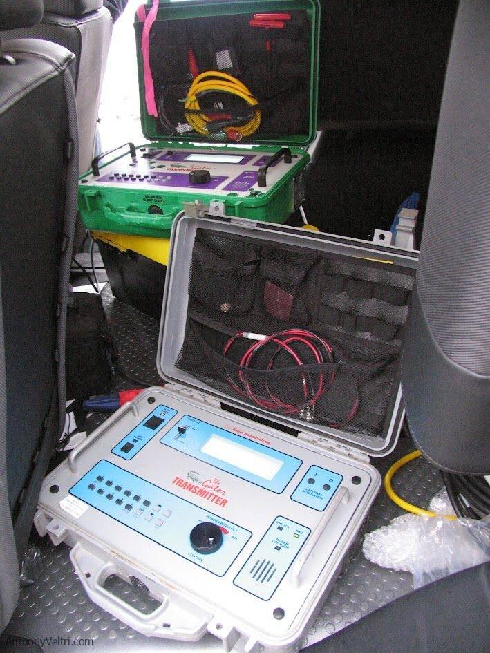
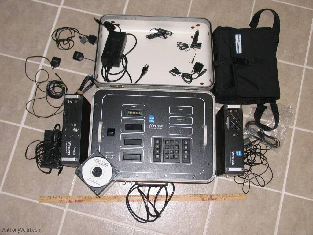
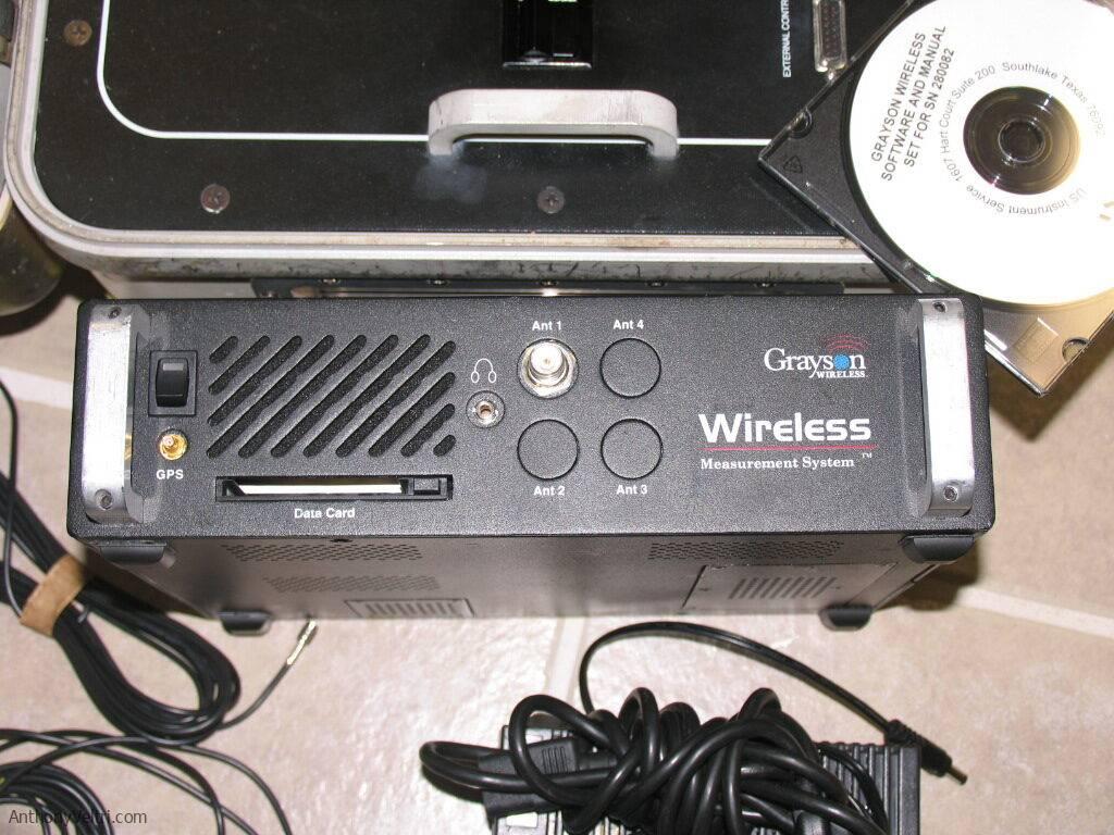
We used a Berkeley Varitronics Systems Gator as the stimulus transmitter (set around 1900 MHz). Our discipline focused on controlling variables:
- Antenna Consistency: We used a known “unity gain” omni stick (2 to 3 dBi) so that comparisons across sites were meaningful.
- Hardware Integrity: We used calibrated 50-ohm coax and high-quality connectors to ensure losses were predictable.
- Backups: We carried duplicates of everything so a field failure never forced an “improvisation” that would ruin the dataset.
The CW drive test workflow: what happened at each site
Each proposed site followed a repeatable routine:
- Deploy mast and mount the omni transmit antenna at a consistent height (often in the 30 to 40 ft range, staying below utility lines to match permit constraints).
- Set transmitter frequency and power, then transmit.
- The measurement vehicle ran a magnet-mount receive antenna on the roof.
- They logged GPS coordinates alongside RSSI (Received Signal Strength Indicator) at frequent intervals.
- They drove outward until the signal truly disappeared, then kept going another short stretch before turning around.
- They repeated the same thing in the opposite direction.
If there were intersections, they took them. The goal was practical reach along public roads, not theoretical circles on a map.
The output was plain and useful: geotagged RSSI traces that showed where coverage fell apart in the real world.
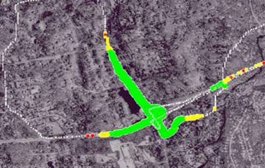
The reach per site was often short by design (sometimes less than a mile). That was the constraint we were working within. In several locations, the Dunkelberger bridges would have been the ideal propagation points for the system. However, the aesthetic requirement was absolute: we could not mount hardware to the historic concrete.
The drive test allowed us to prove exactly where the signal died behind those bridges and identify the specific utility poles needed to work around them. The value was not in rejecting sites. The value was in proving the entire distributed system would provide continuous coverage before a single bracket was mounted.

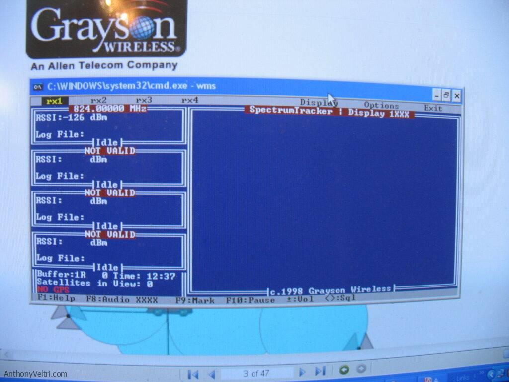
A selection of field measurements from the Merritt Parkway DAS project. These artifacts document The Drill (Stage 3) required to convert the stored sentences of a propagation model into the working capability of a committed infrastructure build (collecting evidence to bridge the Interface Void).
Why the receiver vehicle had to drive “slow, but not randomly slow”

The environment produces two kinds of variation:
- Slow fading (large-scale): terrain, clutter, and shadowing. This is what we want to characterize.
- Fast fading (often Rayleigh): rapid variation from multipath over short distances. This is what we want to average out.
That is why speed mattered. The receiver has to sample fast enough over a short travel distance to compute a stable local mean that filters the fast fading.
This is commonly described with Lee’s criteria (40 lambda averaging): gather enough samples over a distance of 40 wavelengths and average them to reduce fast fading while preserving the slower terrain-driven behavior.
So the measurement crew was trying to drive:
Slow enough to satisfy sampling requirements.
Steady enough to make the averages meaningful.
Safely, while moving slower than normal traffic.
That is why it looked like it took forever. It was not inefficiency. It was measurement integrity.
Analysis and communication: ArcGIS for engineering, Google Earth for humans
We processed the data in Esri ArcGIS Desktop (I think it was ArcGIS 8, but I will not swear to the exact version). It was great for structuring the points and traces, comparing sites, and building layers.
But Google Earth was the killer app for stakeholder understanding. It let non-GIS people interact with the results in context, in the landscape, without needing a GIS workflow.
That became a lasting lesson for me: the analysis tool is not always the communication tool.
The part nobody expects: invisible infrastructure in affluent neighborhoods
Across hundreds of test sites in affluent Connecticut neighborhoods, I was asked what I was doing exactly once.
A cop pulled up alongside me, smacking one of those round Tootsie Pop lollipops. He very casually asked what I was doing. I told him we were taking measurements for the town. He said “okay, be safe,” put the lollipop back in his mouth, and drove off.
That was it. No residents came out to ask questions. No curtain-twitching neighbors. Nothing. We’d be on site for 20 to 45 minutes with a 30-foot mast and vehicles blocking part of the street, and people just drove around us like we were invisible.
I don’t know if that’s typical of very affluent neighborhoods, but I suspect if this work had been in more modest areas, there would have been far more interest in what the heck was going on.
This work also exposed me to the policy and economics behind wireless: spectrum licensing, geographic constraints, and permit realities. The signal is physics. The ability to use the signal is governance. And sometimes governance means 30-foot poles instead of 150-foot towers because that’s what the zoning boards in multiple New England municipalities will permit.
Doctrine alignment
This field note plugs into a few patterns I keep seeing:
Model vs reality: A model is a hypothesis generator. Ground truth is the decision gate.
Two lanes: Innovation Lane creates fast learning and safe experimentation. Production Lane installs with confidence.
Decision latency kills value: Faster validation reduces time from proposed site to committed build.
Objection check
“Why not trust the propagation model?” Because the real world is not just topography. It is clutter, multipath, odd obstructions, and local quirks block by block. Ground truth exists because people have been burned by skipping it.
“Isn’t this just a clever hack?” The mast was the tactic. The capability was repeatable measurement with controlled variables across many candidate sites, fast enough to keep the project moving.
Closing question
Where in your world are you treating a model like an answer (and paying the re-learning tax later) because you skipped the ground truth step? Are you building a system based on “what should be,” or are you building for the reality of the ground?
Technical Notes for the Curious (here be dragons)
Distributed vs centralized coverage
A single 150-foot cell tower might provide coverage for several miles in multiple directions. Drive testing that site means covering a large area with a dense road network, which takes time even with good equipment. The validation task is proving that one site works across its designed coverage area.
A distributed antenna system using 30-foot pole mounts inverts the problem. Each site covers maybe a mile or less. The validation task becomes proving that the collective system provides continuous coverage across all the sites. You’re not testing one large footprint. You’re testing dozens of small overlapping footprints to ensure there are no gaps.
This changes the drive test workflow completely. Instead of one long, comprehensive drive test, you need many short tests with consistent methodology so the results are comparable site to site. The pneumatic mast was optimized for this pattern: fast deployment, quick validation, move to the next site.
Fast fading vs slow fading
When you measure RSSI in a moving vehicle, the signal varies constantly. Some of that variation is meaningful (you drove behind a building, the terrain changed). Some of it is noise you want to filter out.
Fast fading comes from multipath: the signal bounces off cars, buildings, and other objects, arriving at your receiver from multiple directions with different delays. These reflections interfere constructively and destructively, causing rapid signal variation over short distances. At 1900 MHz, you can see 20-30 dB swings in signal strength within a few feet of travel.
Slow fading comes from large-scale effects: terrain shadowing, building obstruction, distance from the transmitter. This is what you actually want to characterize because it determines coverage in the real world.
The averaging process filters the fast fading while preserving the slow fading trends. That’s why the measurement vehicle had to maintain specific speeds and sampling rates. Too fast and you under-sample the fast fading. Too slow and the workflow becomes impractical. The goal is a stable local mean that reflects actual coverage, not multipath artifacts.
Lee criteria (40 lambda averaging)
The commonly cited rule is to average RSSI measurements over a distance of 40 wavelengths to reduce fast fading to acceptable levels (often cited as reducing variation to within 1 dB or so of the true local mean).
At 1900 MHz, the wavelength is about 6.3 inches. Forty wavelengths is roughly 21 feet. So the measurement vehicle needs to collect enough samples over approximately 20 feet of travel to compute a reliable average.
This translates to practical constraints: driving speed, GPS sampling rate, and receiver logging intervals all have to align. Drive too fast and you don’t get enough samples per 20-foot segment. Drive too slow and you’re crawling through neighborhoods for hours. The measurement crew was balancing sampling requirements against operational reality.
The “40 lambda” figure is not magic. It’s an empirical guideline that works well in typical environments. Different environments or different confidence requirements might justify different averaging distances, but 40 lambda is a reasonable starting point.
Why high-gain “omni” can be a trap
An omnidirectional antenna radiates equally in all horizontal directions, which sounds perfect for coverage testing. But “omni” only describes the horizontal plane. The vertical radiation pattern matters just as much.
Higher gain omnidirectional antennas achieve their gain by concentrating energy into a narrower vertical beamwidth. A unity-gain (0 dBi) omni might have a fairly wide vertical pattern, radiating energy from near the horizon up to fairly high angles. A 6 dBi omni achieves higher gain by squeezing that pattern into a thinner vertical slice, concentrating more energy toward the horizon.
In drive testing, this creates problems. Your measurement vehicle is rarely at exactly the same elevation as your transmit antenna. You’re going up and down hills, driving through valleys, testing coverage in neighborhoods at different elevations. A high-gain omni with a narrow vertical beamwidth might show excellent signal on flat terrain but terrible signal when there’s any elevation difference between transmit and receive antennas.
That’s why we used a modest antenna (2-3 dBi range). It maintained reasonable vertical coverage so elevation changes didn’t dominate the measurements. The goal was characterizing horizontal reach and obstruction effects, not fighting antenna pattern artifacts.
Cable loss and consistency
Coaxial cable has loss that increases with frequency. At VHF frequencies (30-300 MHz), cable loss is modest and often negligible for the short runs used in mobile setups. At UHF and higher (like our 1900 MHz work), cable loss becomes significant.
LMR-400 coax, a common choice for this kind of work, has about 6.6 dB of loss per 100 feet at 1900 MHz. If you’re running 20 feet of cable from your transmitter to your antenna, that’s roughly 1.3 dB of loss. If your cable is damaged, has a bad connector, or you accidentally substitute a different cable type, that loss changes and your measurements are no longer comparable site to site.
This is why the Navy Chief’s guidance about connector cleanliness and careful handling mattered so much. A dirty connector might add 0.5 to 1 dB of loss. That doesn’t sound like much, but when you’re trying to compare RSSI measurements across 30 sites, that variability corrupts your dataset. You can’t tell if signal differences are due to site characteristics or equipment inconsistency.
The discipline was simple: use the same cables, keep connectors clean, handle connections carefully, and carry backups so you never have to improvise with whatever cable happens to be in the truck.
Receiver integrity
A receiver in a drive test setup has to handle a wide range of signal levels without distorting the measurements. Strong signals near the transmitter can’t saturate the receiver. Weak signals far from the transmitter need to stay above the noise floor. And there’s always the possibility of interference from other RF sources.
Blocking happens when a strong out-of-band signal reduces the receiver’s sensitivity to the desired signal. You might be trying to measure a weak signal at 1900 MHz while a nearby FM radio station or public safety transmitter is hitting your receiver with a strong signal at a different frequency. Even though you’re not trying to receive that signal, it can reduce your receiver’s ability to accurately measure the signal you care about.
Saturation happens when the desired signal itself is so strong that it overloads the receiver’s front end. This typically happens very close to the transmitter. The receiver stops providing accurate RSSI readings because it has exceeded its dynamic range.
Intermodulation products happen when multiple strong signals mix in the receiver’s non-linear components, creating false signals at frequencies that weren’t actually transmitted. In a dense RF environment, this can create phantom signals that corrupt your measurements.
Quality measurement receivers have high dynamic range, good filtering, and protection circuits to minimize these effects. But they’re still a concern in real-world drive testing, especially in urban or dense RF environments. The measurement crew had to be aware of potential interference sources and validate that their measurements reflected actual coverage, not receiver artifacts.
Speed discipline
The sampling requirements sound simple: collect enough samples over roughly 20 feet of travel to average out fast fading. But translating that into actual driving speed requires balancing multiple constraints.
The receiver logs RSSI at a fixed rate, typically once per second or faster (faster in our case, but the math below keeps it at 1 sample per second). GPS position updates at a similar rate. If you’re driving 20 miles per hour (about 29 feet per second), you’re traveling almost 30 feet between samples. That’s already close to the 20-foot averaging window, giving you barely two samples to average. Drive faster and the problem gets worse.
Slow down to 10 mph and you’re traveling about 15 feet per second, giving you better sampling density. Slow down to 5 mph and you’re crawling, which creates its own problems: frustrated drivers behind you, safety concerns when you’re moving much slower than traffic expects, and workflow collapse when it takes an hour to validate a site that should take 20 minutes.
The measurement crew had to find the speed that satisfied sampling requirements while remaining safe and practical. That typically meant 10-15 mph on residential streets, slower on complex routes with turns, and coordinating with local traffic patterns to avoid creating hazards.
This is why “they have to drive slow” was an incomplete understanding. They had to drive at a specific controlled speed that balanced technical requirements, safety, and operational efficiency. That’s a much harder discipline than just “slow.”
Last Updated on March 15, 2026